 QuickPLS
What the method does
Fuzzy-set qualitative comparative analysis examines necessary and sufficient set relationships. Conditions and outcomes are represented by memberships between 0 and 1, based on substantive definitions and calibration. A truth table organises configurations; logical minimisation identifies simplified pathways under stated assumptions. Different pathways can lead to the same outcome, and outcome absence requires its own analysis.
AND: min(Aᵢ, Bᵢ). OR: max(Aᵢ, Bᵢ). NOT A: 1 − Aᵢ. Sufficiency consistency: Σᵢmin(Xᵢ,Yᵢ) / ΣᵢXᵢ.
Xᵢ is case i’s membership in a condition or configuration and Yᵢ its outcome membership. Consistency describes the degree to which X is a subset of Y. Coverage uses ΣᵢYᵢ as the denominator and describes how much of the outcome the pathway covers. These ratios require nonzero denominators.
Data and analysis in QuickPLS
Use one case per row, a case identifier, condition columns and an outcome. Inputs may be raw values with justified calibration or existing memberships in [0,1]. Define missing-value and exact-crossover decisions explicitly.
QuickPLS supports calibration, necessity checks, truth tables, solutions and case inspection for your suitable data. The exercise below uses a small downloadable membership file so you can follow each decision and calculation.
Follow a worked example
The following example shows the data, settings and decisions for one analysis. Use the linked practice files to follow it. For your own study, keep the procedure and choose the variables, model and settings that fit your research question.
Download memberships.csv to begin. It contains 10 rows and 5 columns. The example below identifies the variables to use, their roles and any rows to exclude; not every column is an analysis variable.
Study question and analytical approach
Which combinations of capacity, reach and coordination are associated with successful project delivery? This example uses fuzzy-set Qualitative Comparative Analysis (fsQCA) to examine that question in a small synthetic dataset. It follows the analysis from the original cases to a solution that can be checked by counting.
fsQCA represents each case as a member of defined sets, such as high capacity and successful delivery. A condition is an explanatory set; a configuration is a combination of conditions. The method examines whether particular configurations are sufficient for the outcome and whether individual conditions are necessary. Several sufficient pathways can coexist.
Set membership expresses the extent to which a case belongs to a defined set, rather than its probability of success. Calibration establishes that membership from a measurement and a substantive definition. The first exercise uses memberships already supplied with the data; a separate raw-score exercise is available for practising calibration.
Dataset and set definitions
The ten invented community projects in memberships.csv have four set variables: A denotes high capacity, B broad reach, C strong coordination and Y successful delivery. case_id identifies the project. The condition order is A, B, C throughout the walkthrough.
The file contains memberships rather than raw survey responses. Values of 1 and 0 indicate full membership and full non-membership respectively. Analyse the presence of successful delivery. The exercise examines how the three conditions combine, including whether a condition can be required for success without being sufficient on its own.
The set names provide a teaching interpretation of the values. They do not come from an empirical community-project study or establish a causal relationship.
Open the exercise and identify the correct file
The saved Guided fsQCA project contains the membership and raw-score exercises, with saved results from the 1.03.07 sample programme. Open a copy for practice and retain the original. To work from a CSV, use memberships.csv for the walkthrough on this page.
The separate raw-scores.csv file is for calibration practice. Its columns and results belong to that study; use memberships.csv to reproduce the walkthrough below.
A separate paper-based exercise
The linked paper tutorial offers delivery-memberships.csv as a separate exercise. Its expected expression is capacity AND coordination, OR capacity AND reach. QCA 3.25 and an independent calculation verified those reference answers; the d-case file has not been rerun in QuickPLS for that answer pack. The walkthrough here uses the m-case file.
Memberships, calibration and case eligibility
Define each condition and the outcome before examining a solution. For research data, inspect the measurements, missing values and case population, then justify the calibration from those definitions and relevant case knowledge.
Membership 1 means fully in a set and membership 0 fully outside it. At the crossover, 0.5, the case is neither more in than out nor more out than in. An exact crossover and a missing measurement therefore require different decisions.
Select existing memberships for memberships.csv. Recalibrating these values would change the supplied sets. The separate raw-score file requires its own justified calibration.
The setup image should show Conditions A, B and C, outcome Y, existing memberships and the stated case decisions. An empty form illustrates where controls are located but does not confirm that the exercise is ready to calculate.
Open the fsQCA calculation
Import the membership exercise
In a writable project choose File > Import Data…, then Choose data file…. Select memberships.csv, inspect Review & import and choose Import dataset. Confirm the imported file has ten cases and columns case_id, A, B, C and Y.
What you should see: The imported file has ten rows and case_id, A, B, C and Y.
How to read it: Treat A, B, C and Y as existing memberships; do not calibrate them again.
Open the dataset-based method
Select the imported dataset, choose Calculate… and find Fuzzy-set Qualitative Comparative Analysis. Open Method settings. This method uses the dataset, so an empty structural-model canvas is expected.
What you should see: The fsQCA settings are linked to the selected dataset.
How to read it: No structural path diagram is needed for this dataset-based calculation.
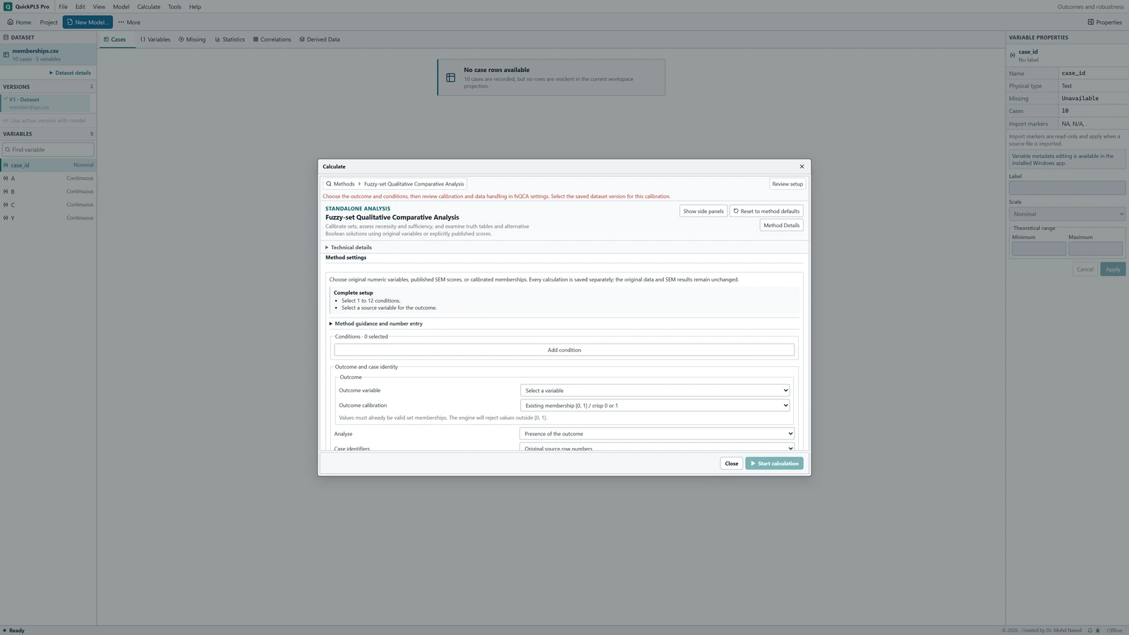
Fuzzy-set Qualitative Comparative Analysis settings in QuickPLS. Select your own dataset and model, then use the choices described in the steps. Keep the baseline identifiable
Each completed calculation has its own saved result. Keep a note of which result uses the baseline settings and which changes a threshold so you can return to the intended calculation.
What you should see: Baseline and changed-threshold calculations have separate saved results.
How to read it: Read each solution with the settings and case decisions from its own calculation.

Select the sets and resolve the two exceptional cases
Under Method settings add A, B and C as Conditions, in that order. Select Y as Outcome variable, Presence of the outcome as Analyse and case_id as Case identifiers. For every selected column choose Existing membership [0, 1] / crisp 0 or 1; these values must not be recalibrated.
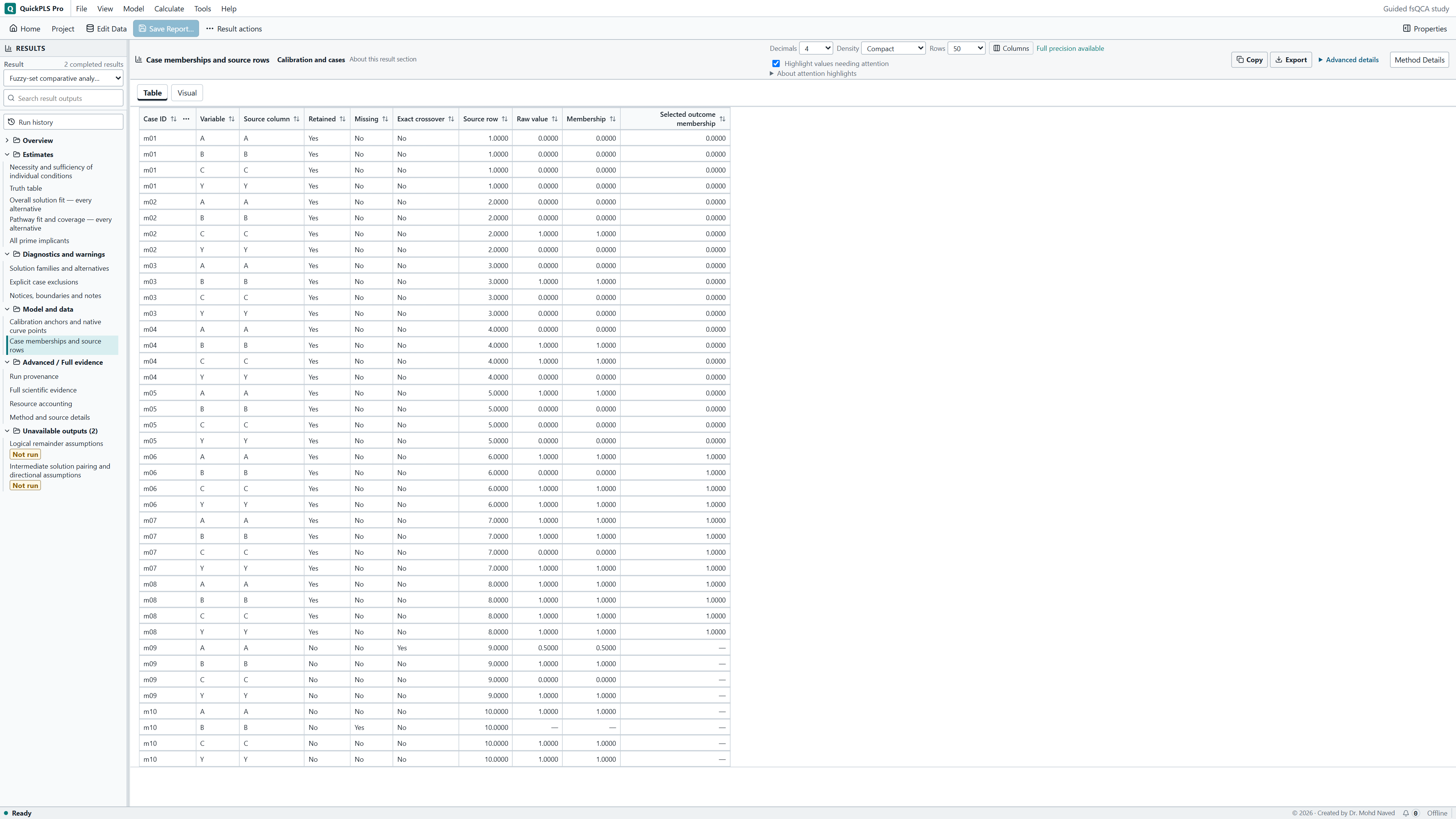
Case m09 has A = 0.5, exactly at the crossover. Case m10 has a missing B value. For this baseline, explicitly exclude both and record the separate reasons. The analysed sample consists of eight cases, m01 to m08. This is an exercise-specific rule; a research study needs a case policy justified by its measurements and design.
Expand Data: missing values and exact crossovers. Set Missing selected values to Exclude affected cases and record every exclusion; this excludes m10 because B is missing. For m09, enter 9 in Source row to exclude, enter the reason A is exactly 0.5, and choose Record deliberate crossover exclusion. Row 9 is the source data row for m09 in the supplied CSV, not the ninth line including its header. The intended result includes m01 to m08.
Calculate the baseline truth table and solution
Confirm the selected data
Check memberships.csv and the set assignments described above. The separate raw-scores.csv file is a different calibration exercise.
What you should see: The selected file contains memberships A, B, C and Y with m-case identifiers.
How to read it: Use existing memberships rather than recalibrating them.
Check case eligibility
Expand Data: missing values and exact crossovers. Set Missing selected values to Exclude affected cases and record every exclusion; this excludes m10 because B is missing. For m09, enter 9 in Source row to exclude, enter the reason A is exactly 0.5, and choose Record deliberate crossover exclusion. Row 9 is the source data row for m09 in the supplied CSV, not the ninth line including its header. The intended result includes m01 to m08.
What you should see: m09 and m10 are excluded for the stated distinct reasons; m01 to m08 remain.
How to read it: A crossover is not the same as missing data.
Run the baseline
Set Frequency threshold to 1, Consistency threshold to 0.80 and PRI threshold to 0.50 under Truth table and solution assumptions. Leave Request intermediate solutions with explicit directional expectations unchecked for the baseline. Choose Start calculation and wait for completion.
What you should see: The completed baseline records frequency 1, consistency 0.80 and PRI 0.50.
How to read it: A later threshold change needs a new calculation.
Read the completed calculation
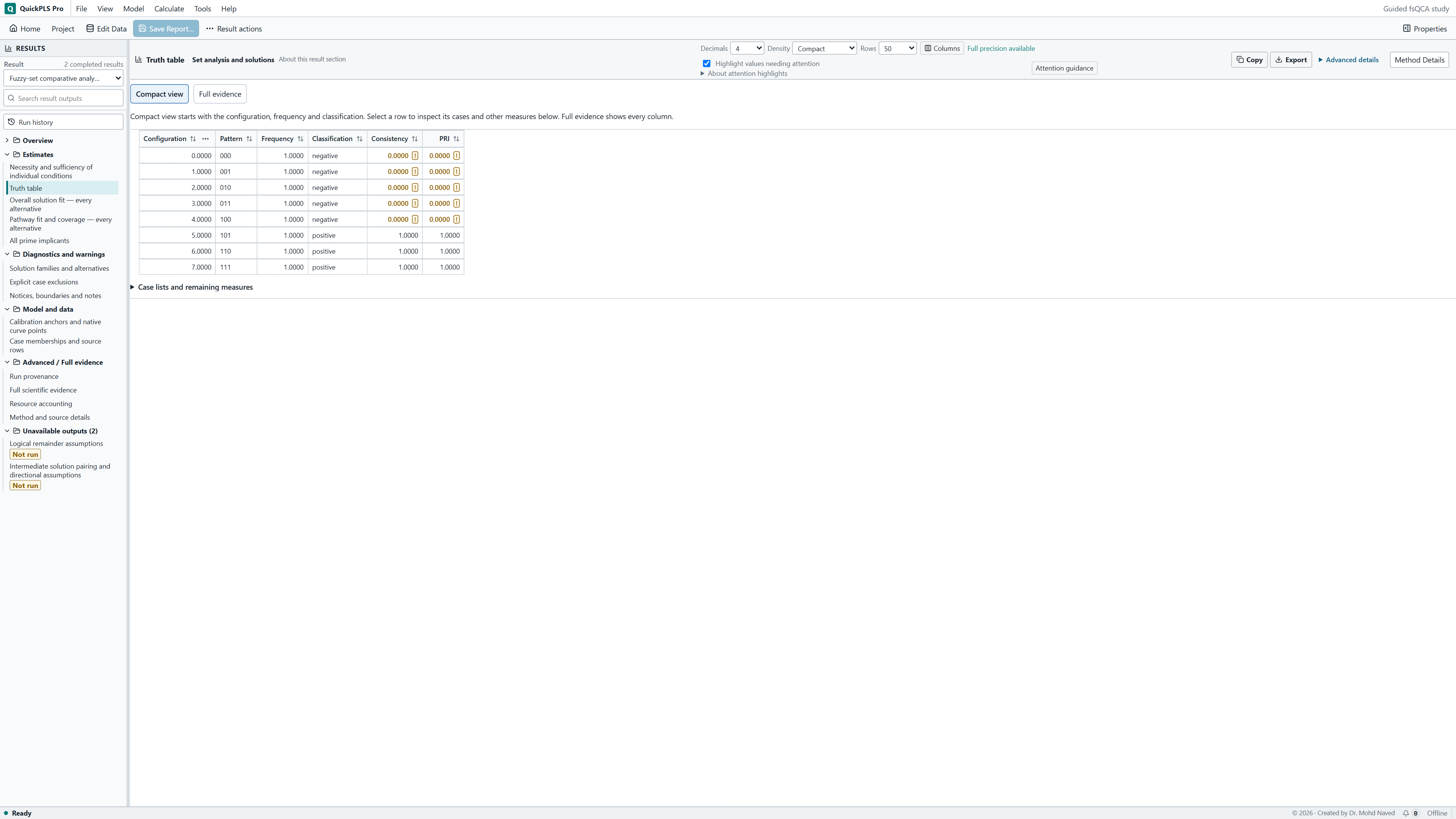
In Results, use Result to select the completed membership calculation. Open Estimates > Truth table. Then read the conservative rows in Overall solution fit — every alternative and Pathway fit and coverage — every alternative, keeping the same Family and Solution identifiers together. Open Model and data > Case memberships and source rows to locate the original m-cases.
What you should see: The truth table and solution tables belong to the same completed baseline.
How to read it: Match family and alternative identifiers before interpreting coverage.
Interpret the truth table and solution alternatives
The truth table groups cases by the presence or absence of the conditions. Inspect each row's case count, outcome consistency and original cases. PRI provides an additional sufficiency check for configurations that also fit the absence of the outcome; it should be interpreted with consistency and the case pattern.
A solution simplifies the configurations under the chosen rules for unobserved combinations. Each alternative is a complete expression. Analyse alternatives separately, since selecting terms from different alternatives creates an expression that was not the reported solution.
Consistency measures how closely the cases conform to the proposed set relationship. Sufficiency coverage measures how much of the outcome is covered by a pathway or by the whole solution. Neither statistic is a regression coefficient or a causal effect size.
Use Case memberships and source rows to locate m05, m06, m07 and m08. Their original memberships explain why capacity alone is insufficient and why the two pathways overlap. The worked numbers below belong to these m-cases.
On a small screen, swipe the table sideways to see every column.
| Output | How to read it | What to check |
|---|---|---|
| Truth table | The observed condition combinations, their case counts and evidence of sufficiency. | Check contradictory cases, missing values and cases exactly at the crossover. |
| Solution alternatives | Separate simplified explanations under the chosen rules for unobserved combinations. | Do not merge alternative solutions into one expression. |
| Consistency and coverage | How closely the relationship holds and how much of the relevant set it covers. | Neither is a regression coefficient or a causal effect size. |
Solution notation and omitted conditions
Notation example
A*B + C*D means (A AND B) OR (C AND D). Each conjunction is a pathway; the plus sign joins them into a solution. A condition explicitly marked absent must be absent in that pathway. An omitted condition is unrestricted within the term. Examine the cases covered by each term before interpreting its substantive meaning. This expression illustrates notation rather than a software benchmark.
Verify the solution and its coverage
The eight included cases have 0 or 1 memberships. The successful cases are m06 = 101, m07 = 110 and m08 = 111, with digits ordered A, B, C. Every success has A and at least one of B or C.
The resulting expression is A AND (B OR C), equivalently A*B + A*C: capacity with reach, or capacity with coordination. A*B covers m07 and m08; A*C covers m06 and m08.
Each pathway covers two of the three successful cases, giving raw coverage 2/3. Raw coverage includes m08, which belongs to both pathways. Each pathway also contributes one successful case not covered by the other, giving unique coverage 1/3.
The union covers all three successful cases and no unsuccessful cases. Solution consistency and solution coverage are therefore both 1. These counts agree with the saved result for memberships.csv.
Reference answers for the separate d-case exercise
For the separate delivery-memberships.csv answer pack, the successful cases are d06, d07 and d08. Its independently checked solution consistency, coverage and PRI are 1. Capacity alone has sufficiency consistency 0.75 and necessity consistency 1. These reference values belong to that d-case file, not to a newly executed QuickPLS analysis.
Explain necessity and sufficiency through the cases
Inspect m07 and m08 under the A*B pathway. C is absent in m07 and present in m08, so this term leaves C unrestricted. Coordination still contributes to the other pathway, A*C; its omission from A*B does not make it irrelevant to the solution.
Case m05 has A = 1, B = 0, C = 0 and Y = 0. It has capacity without reach or coordination and does not succeed. This counterexample shows why capacity alone is insufficient.
Capacity occurs in four included cases, of which three succeed, giving sufficiency consistency 3/4. Every successful case has capacity, so it is necessary within this dataset. Necessity asks whether success requires the condition; sufficiency asks whether the condition or combination is enough for success.
In an empirical analysis, relate supporting and contradictory cases to their substantive records. The logical expression identifies the pattern to explain; case knowledge and research design determine the explanation it can support.
Sensitivity to consistency and frequency thresholds
Run a separate calculation that raises consistency from 0.80 to 0.90 while keeping the other baseline settings. The successful configurations remain above either consistency threshold; the unsuccessful configurations remain below both. Their positive classification should therefore be unchanged.
In another calculation, restore consistency 0.80 and set frequency to 2. Each configuration occurs only once, so no row meets the revised minimum. The resulting empty solution follows from the frequency rule and case distribution.
These changes address different questions: consistency concerns agreement with the outcome, while frequency concerns the number of cases behind each row. Keep the baseline result and record the changed setting alongside each new result.
For research data, justify alternative thresholds and calibrations from the set definitions and case population. Explain which pathways, cases and conclusions change, including changes that weaken the proposed explanation.
Diagnose a result that differs from the baseline
First compare the dataset, case decisions, outcome direction and thresholds with the baseline. This membership exercise uses m-cases; the separate paper exercise uses d-cases and the raw-score calibration exercise uses r-cases. Their values cannot be substituted for one another.
Compare logical expressions by their meaning as well as their printed order. Reordering conditions within a conjunction does not alter the pathway. The table identifies setup differences that do change the analysis and explains how to resolve them.
On a small screen, swipe the table sideways to see every column.
| What you notice | What to check | What to do |
|---|---|---|
| Ten cases enter the calculation | Whether m09 and m10 received explicit case decisions | Apply the stated crossover and incomplete-case exclusions, then calculate again. |
| The truth table uses raw-score calibration | Whether you selected raw-scores.csv instead | Return to memberships.csv and choose existing memberships. |
| No positive configuration remains | Whether minimum frequency is 2 | Restore frequency 1 for the baseline; keep the frequency-2 result as a separate sensitivity check. |
| Pathway coverage seems to add to more than 1 | Whether m08 belongs to both pathways | Use unique coverage to identify non-overlapping contributions and solution coverage for their union. |
Report the worked analysis
Identify memberships.csv and the completed baseline calculation in the report. State the solution family, the complete alternative selected and any assumptions about unobserved combinations.
Results example: Successful delivery in the synthetic cases was covered by capacity combined with reach or capacity combined with coordination. Each pathway had consistency 1 and raw coverage 0.667. Their overlap left each with unique coverage 0.333. Together they covered all three successful cases.
The table retains exact fractions for checking the rounded coverage values. If other complete alternatives are reported, present them separately with their own fit and case interpretation.
| Item to report | Value in this exercise |
|---|---|
| Included cases | 8 of 10 |
| Positive configurations | 101, 110, 111 |
| Expression | A* |
| Solution consistency; coverage | 1; 1 |
| Each pathway: raw; unique coverage | 2/3; 1/3 |
Methods example: synthetic membership data
We analysed capacity, reach and coordination using existing set memberships. We excluded one case at the crossover and one with a missing condition, leaving eight cases. The baseline used frequency 1, consistency 0.80 and PRI 0.50. We inspected the complete truth table and the cases supporting each pathway.
Reporting an empirical fsQCA study
- Define each condition and outcome, identify the source of its values and explain the calibration anchors. State the included cases and the reasons for exclusions or separate treatment.
- Report frequency, consistency and PRI thresholds, together with the outcome direction. Frequency counts cases assigned to a truth-table row; PRI helps assess whether a row fits both the outcome and its absence.
- Name the solution family, directional expectations and assumptions about unobserved combinations. Present complete alternatives, pathway and solution coverage, and the cases supporting the interpretation.
Scope of the interpretation
The exercise has a transparent binary case pattern. Fuzzy memberships and unobserved configurations require additional interpretation of calibration, consistency and simplifying assumptions. A solution alone does not establish a causal mechanism.
Analyse outcome absence as a separate question, since the combinations associated with failure need not be the inverse of those associated with success. Original variables or explicitly published score datasets may be used if their measurement and calibration are explained.
Record the rule for exact .5 memberships. Moving a borderline value to a preferred side of the crossover changes the evidence and must not be treated as an inconsequential numerical adjustment.
Exercises and saved analysis record
Use the original cases to explain why the two raw coverages cannot be added, why m09 requires a separate decision and why frequency 2 changes the solution. Identify the unsuccessful high-capacity case before consulting the solution table.
Save the project after the baseline and sensitivity calculations, then reopen it. Verify that you can select each completed result and recover its case decisions, thresholds and complete solution. Keep those details with the exported report.
- Locate m05, m06, m07 and m08 and explain how they distinguish necessity, sufficiency and overlapping pathways.
- Define condition, configuration and solution pathway using this dataset.
- Record the exact data file and completed calculation in the exported report.