 QuickPLS
What the method does
A truth table lists combinations of condition presence and absence. Frequency, consistency and the selected outcome rules determine which observed rows enter minimisation. Contradictory rows and unobserved configurations require different treatment: a contradiction contains conflicting evidence, while an unobserved configuration contains no observed case.
k binary conditions give 2ᵏ possible configurations.
A configuration is a pattern such as A present, B absent and C present. The condition order determines how a binary pattern is read. Fuzzy memberships also contribute to set-fit measures; the configuration label alone does not contain every case value.
Data and analysis in QuickPLS
Use calibrated conditions, an outcome and case identifiers. Define frequency, consistency and PRI thresholds before interpreting row classification.
QuickPLS builds the truth table and provides case memberships and row diagnostics. Read the configuration order and inspect the contributing cases before changing a threshold.
Follow a worked example
The following example shows the data, settings and decisions for one analysis. Use the linked practice files to follow it. For your own study, keep the procedure and choose the variables, model and settings that fit your research question.
Download memberships.csv to begin. It contains 10 rows and 5 columns. The example below identifies the variables to use, their roles and any rows to exclude; not every column is an analysis variable.
A row represents a combination of conditions
A truth table groups cases by their condition combinations, called configurations. With three binary conditions there are eight possible combinations. Several cases can share one combination, and another combination may have no cases at all. A truth-table row is therefore not the same thing as a row in your original dataset.
Read three measures together. Frequency counts the cases assigned to the combination. Consistency measures how closely membership in that combination stays within membership in the outcome. PRI, or proportional reduction in inconsistency, helps check whether an apparent relationship with the outcome also overlaps with its absence. None of these measures is a probability that your explanation is true.
Agree what the memberships mean before reading the table
Save the chosen conditions, outcome and calibration, meaning the rules that translate measurements into membership of a set. Record how you will handle missing values and exact crossover memberships. A crossover is the point of maximum uncertainty about whether a case belongs to a set. These choices determine which cases and memberships the truth table will use.
Open and investigate the truth table
Choose the settings
Open Calculate… > Fuzzy-set Qualitative Comparative Analysis. Under Method settings confirm the conditions, outcome, calibration and case decisions.
Set the thresholds
Enter Frequency threshold, Consistency threshold and PRI threshold under Truth table and solution assumptions. Record the reasons for these choices with your analysis notes.
Calculate and open the table
Choose Start calculation. When it completes, select the result and open Estimates > Truth table. This table belongs to the completed calculation; compare it with the settings used for that run.
Check cases against configurations
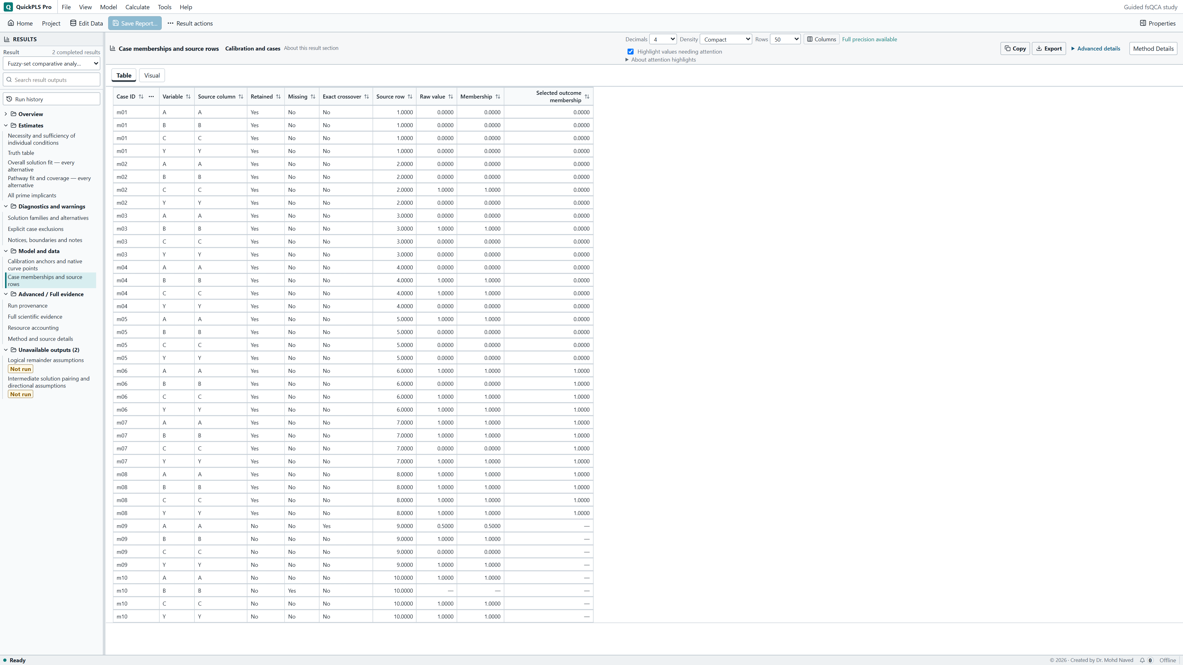
Read the condition order before interpreting a pattern. Use Model and data > Case memberships and source rows to find the original cases and compare them with the configuration.
Calculate a changed setup separately
After changing calibration, exclusions or thresholds, start a new calculation and select its completed result. Keep the baseline result for comparison; a table from an earlier calculation cannot show a later settings change.
Use a surprising row as a reason to inspect its cases
The thresholds decide which rows qualify for the next step, minimization. Minimization simplifies eligible combinations into pathways. Frequency 1, consistency .80 and PRI .50 make the small exercise below easy to check. They are teaching choices, not recommended cutoffs for every dataset.
Look closely at rows with little case support, conflicting outcomes or unexpected memberships. A display filter changes what is visible. Changing calibration, exclusions or cutoffs changes the analysis and requires a new calculation. Keep different situations distinct: no observed cases, cases deliberately excluded, and a measure that cannot be calculated are not all zero.
If a combination contains both successful and unsuccessful cases, open those observations. Check coding, set definitions and context before deciding what the disagreement means. An undefined measure also needs its own explanation; it does not establish that the combination never occurs.
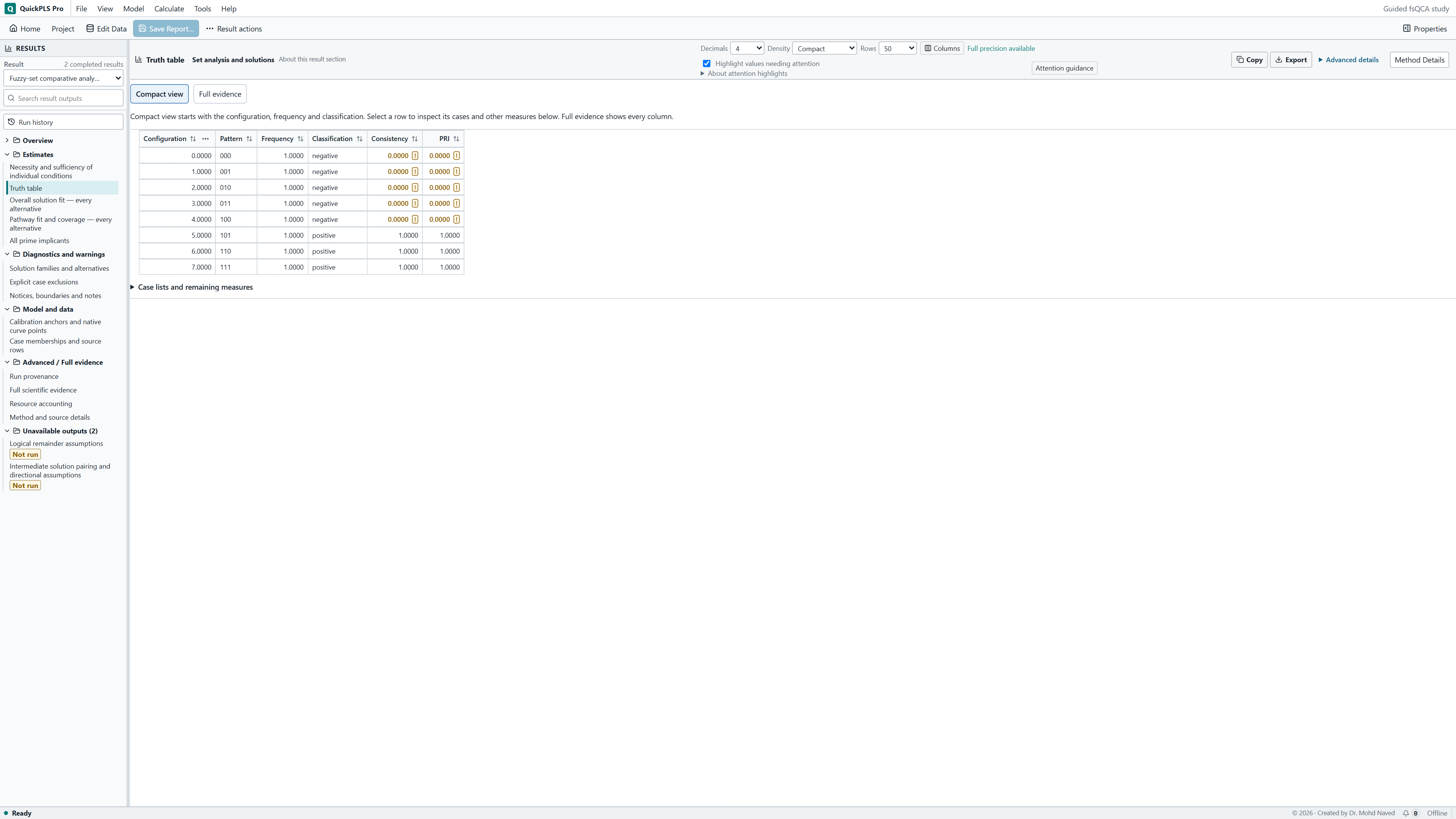
For this exercise, the completed Truth table should show configurations in the A, B, C order. Compare its case frequencies with the eight included source cases in the table below. A different two-condition example cannot verify these counts.
On a small screen, swipe the table sideways to see every column.
| Output | How to read it | What to check |
|---|---|---|
| Frequency | Read the number of included cases assigned to the configuration alongside the selected minimum. | Membership sums and configuration frequency are different quantities. |
| Consistency and PRI | Read sufficiency consistency and PRI for the selected outcome, whether presence or absence. | A high consistency alone may conceal overlap with outcome absence. |
| Row classification | Use the saved cutoffs to distinguish positive configurations, contradictory configurations and logical remainders. | A remainder is not an observed negative case; changing cutoffs changes the specification. |
| Included and excluded cases | Trace a row back to original cases and record reasons for omission. | Do not adjust calibration or remove a case merely to improve its classification. |
Build the delivery table from the original cases
In the delivery exercise, A means capacity, B reach and C coordination. A combination such as capacity present, reach absent and coordination present becomes one truth-table row. The table shows whether that combination occurs, how many cases have it and how those cases relate to delivery, the outcome Y. Three binary conditions give eight possible combinations.
Open memberships.csv. For this baseline, explicitly exclude m09 because A = 0.5 and m10 because B is missing. The other eight cases supply every binary combination once. These exclusions are stated decisions for the exercise. They let you learn the complete table before handling sparse or contradictory evidence in a research dataset.
Ask a different question of each measure
Frequency asks how many cases are assigned to this combination, regardless of their outcome. Consistency asks how well the combination fits inside the outcome set. PRI asks whether the apparent sufficiency relationship also overlaps with outcome absence. A large number of cases does not guarantee good consistency, and a high consistency value does not create evidence for a combination that has never been observed.
Use frequency 1, consistency 0.80 and PRI 0.50, with no contradiction band. Every included combination has one case whose outcome is completely present or absent. That makes the classification easy to inspect. A real study needs its own reasons for the thresholds, based on case support, calibration, contradictory evidence and the research question.
Inspect the cases before simplifying the table
Assign the membership columns
Under Method settings add A, B and C as Conditions, in that order. Select Y as Outcome variable, Presence of the outcome as Analyse and case_id as Case identifiers. For every selected column choose Existing membership [0, 1] / crisp 0 or 1; these values must not be recalibrated.
What you should see: A, B and C are conditions and Y is the outcome, in the stated order.
How to read it: Existing memberships are selected.
Record the case decisions
Expand Data: missing values and exact crossovers. Set Missing selected values to Exclude affected cases and record every exclusion; this excludes m10 because B is missing. For m09, enter 9 in Source row to exclude, enter the reason A is exactly 0.5, and choose Record deliberate crossover exclusion. Row 9 is the source data row for m09 in the supplied CSV, not the ninth line including its header. The intended result includes m01 to m08.
What you should see: The included cases are m01 to m08, with m09 and m10 excluded for different reasons.
How to read it: Check the source rows.
Calculate the table
Set Frequency threshold to 1, Consistency threshold to 0.80 and PRI threshold to 0.50 under Truth table and solution assumptions. Leave Request intermediate solutions with explicit directional expectations unchecked for the baseline. Choose Start calculation and wait for completion. In the completed result open Estimates > Truth table. Read patterns 000 through 111 in A, B, C order.
What you should see: The baseline table has eight observed binary configurations, each with frequency 1.
How to read it: Read classification using the stated thresholds.
Compare neighbouring configurations
Compare 101, represented by m06 with Y = 1, with 100, represented by m05 with Y = 0. Their condition difference is C. Locate both cases in Case memberships and source rows to check their original values.
What you should see: Neighbouring rows differ in the indicated condition.
How to read it: Inspect their original cases before attributing the outcome difference to that condition.
Try a separate threshold calculation
Run a new calculation for each threshold change below and select that completed result. Compare its row classifications with the baseline before interpreting any changed solution.
What you should see: The frequency-2 calculation has its own result.
How to read it: Its lack of qualifying configurations is part of the sensitivity finding.
Check all eight combinations by hand
The table below is counted from the included CSV rows. The successful configurations are 101, 110 and 111. All possible configurations are observed at baseline. A logical remainder is a configuration without enough observed support under the chosen rule. It is not an unsuccessful observed case merely because it was not classified as positive.
When frequency becomes 2, all eight combinations fall below the requirement. Their cases have not disappeared from the file. The classification changes because you now require more support. Parsimonious solutions can use assumptions about remainders to simplify an explanation, so keep a lack of sufficient observed support distinct from observed evidence of failure.
On a small screen, swipe the table sideways to see every column.
| A B C | Original case | Y | Frequency |
|---|---|---|---|
| 000 | m01 | 0 | 1 |
| 001 | m02 | 0 | 1 |
| 010 | m03 | 0 | 1 |
| 011 | m04 | 0 | 1 |
| 100 | m05 | 0 | 1 |
| 101 | m06 | 1 | 1 |
| 110 | m07 | 1 | 1 |
| 111 | m08 | 1 | 1 |
Investigate disagreement instead of hiding it
Every configuration here contains only one binary case. There is therefore no disagreement between cases within a configuration. That tells us little about repeated evidence: the example cannot show whether several cases with the same conditions would consistently have the same outcome.
In a research study, a row may contain cases with different outcomes. Check for data-entry errors, unclear set definitions, meaningful contextual differences or a condition missing from your proposed explanation. Changing a cutoff can change the row's label, but it does not explain the disagreement. Keep an inconvenient case unless you have a research reason for excluding it, and record that reason.
Try one change to consistency and another to frequency
Raise consistency from 0.80 to 0.90 in a separate calculation. The three positive rows already have consistency 1, so they remain positive. This checks one threshold in this file. It does not test different calibration choices or another sample.
In another calculation, restore consistency 0.80 and raise frequency from 1 to 2. No combination has enough cases. Read that change in the completed truth table before interpreting a changed or empty solution. This order helps explain whether the result follows from the rows that qualified for simplification.
Check the row, its cases and the active settings
When the table is surprising, start with its condition order and the original case. Then check exclusions, any display filters and which completed calculation is selected. These checks separate a reading problem from a changed analysis.
On a small screen, swipe the table sideways to see every column.
| Symptom | Check | Action |
|---|---|---|
| A condition order looks reversed | The displayed order of A, B and C | Read every binary pattern in that order before identifying cases. |
| A case appears absent from the result | Its missing-value or crossover decision and any display filter | Check the original row, the case policy and Exclusions before interpreting the table. |
| No row passes frequency | The count in each row and the selected minimum | Use the intended threshold or report that no row has enough cases to meet it. |
| A changed threshold seems to have no effect | Whether a new calculation completed and its result is selected | Start the intended calculation and select its result; an older table keeps its original settings. |
| An unobserved combination is called a failure | Whether any case actually supports that configuration | Describe it as a remainder under the selected rule, not as observed evidence against the outcome. |
Report how rows were classified
Describe the condition order, case decisions and thresholds in Methods. In Results, identify the observed and positive configurations. The example table keeps case counts separate from configuration counts, so a reader can follow how the solution was reached.
| Reporting item | Teaching example |
|---|---|
| Condition order | A, B, C |
| Cases before and after exclusions | 10; 8 |
| Observed configurations | 8 of 8 |
| Positive configurations | 101, 110, 111 |
| Unobserved configurations at baseline | None |
| Frequency-2 sensitivity | No configuration reaches the requirement |
Example Methods paragraph
The synthetic delivery analysis used A, B and C as existing memberships and Y as the outcome. We excluded the explicitly identified crossover and incomplete cases. Each of the eight binary configurations then contained one case. We inspected row membership and used frequency 1, consistency 0.80 and PRI 0.50, with no contradiction band.
Explain the table before opening the solution
For the exercise, you could write: Three configurations were classified as positive, each supported by one successful case. The other five observed configurations contained unsuccessful cases. Increasing consistency to 0.90 left those classifications unchanged; requiring frequency 2 left no configuration with enough cases. Each statement can be checked against the file and the specified rules.
Find m05 and m06 and explain how C distinguishes their configurations. Predict the effect of a higher frequency requirement before running it. A full eight-row table contains every possible combination; it does not mean that every combination is successful. Keep the truth table beside the chosen solution when writing your interpretation.
- Work out how many configurations are possible before judging which are missing.
- Count assigned cases for frequency; do not substitute a sum of fuzzy memberships.
- Save the thresholds and case decisions with the table.
- Use contradictory cases to investigate the explanation, not just to adjust a cutoff.
Explain the thresholds you choose
Frequency 1, consistency .80 and PRI .50 apply to this teaching exercise. In your study, justify the cutoffs using the available cases, measurement choices and research question. The optional contradiction band introduces a lower consistency boundary for identifying contradictory rows; explain that boundary if you use it instead of assuming every study needs one.
In the optional band, the lower boundary is included and the main consistency threshold is the upper boundary, which is not included. Enter the lower value through Contradiction lower boundary after enabling the band. Keep the band disabled for this exercise.
Trace a teaching row back to its cases
Use memberships.csv or a copy of the Guided fsQCA project. The project contains saved teaching calculations from the 1.03.07 sample programme. These are supplied examples, not a fresh calculation in your Store installation or a journal replication. Keep the originals while trying different thresholds.