 QuickPLS
What the method does
An exact binomial check evaluates the number of outcome-positive cases in a crisp configuration against a chosen null probability. It adds a particular statistical diagnostic to the row. It does not replace calibration, logical minimisation or the substantive assessment of the cases.
Upper-tail probability: P(K ≥ k) = Σⱼ₌ₖⁿ choose(n,j)p₀ʲ(1 − p₀)ⁿ⁻ʲ.
n is the number of trials, k the observed successes and p₀ the declared null probability. The binomial interpretation assumes the stated trial model. A one-sided probability must retain its direction and null value.
Data and analysis in QuickPLS
Use eligible crisp 0/1 conditions and outcomes with identifiable cases. Define the success event and null probability before inspecting row probabilities.
QuickPLS reports the exact checks with successes, trials and null probability. Match those counts to the configuration before interpreting the tail probability.
Follow a worked example
The following example shows the data, settings and decisions for one analysis. Use the linked practice files to follow it. For your own study, keep the procedure and choose the variables, model and settings that fit your research question.
Download crisp-outcomes.csv to begin. It contains 10 rows and 5 columns. The example below identifies the variables to use, their roles and any rows to exclude; not every column is an analysis variable.
Ask whether a row's success count is unusual
Suppose every case in a truth-table row has the outcome. That looks consistent, but a row with very few cases can reach that result quite easily. The exact binomial check compares the observed success count with a reference success probability that you choose. It adds a probability calculation beside the crisp truth table; it leaves the original row classifications and simplified solutions unchanged. Choose the reference probability, significance cutoff and minimum case count before reading the result.
Start with a completed Advanced calibration result that used Inclusive crisp calibration for every selected condition and the outcome. Inclusive crisp turns measurements into in-or-out memberships using a stated threshold. A result calculated with Existing membership is a different source type even if all its values are 0 or 1. Check the saved calibration procedure as well as the numbers.
Prepare the source and three decision rules
Use a completed Advanced calibration result with Inclusive crisp calibration for every selected condition and the outcome. Decide p0, the reference success probability; alpha, the cutoff for the resulting probability; and the minimum number of observed cases required for a row. Write down why those choices suit the study before calculating.
Add the separate diagnostic to the crisp result
Choose the source
Open Data, More, Exact binomial checks. Select the saved crisp Source analysis, Owning saved study and Specification revision.
Enter the choices
Click Load binomial choices. Set Null inclusion threshold for p0, Significance level for alpha and Minimum observed frequency for the case-count rule.
Verify and preview
Click Verify crisp source and choices. Resolve any eligibility message, then click Preview native binomial diagnostics and inspect the proposed row calculations.
Save the diagnostic setup
Click Save binomial revision so the selected probability and frequency rules remain attached to the study.
Calculate and inspect
Click Calculate and retain binomial diagnostics. Read each row's successes, case count, probability and decision together, then keep the matching report with its source analysis.
Read the probability together with the number of cases
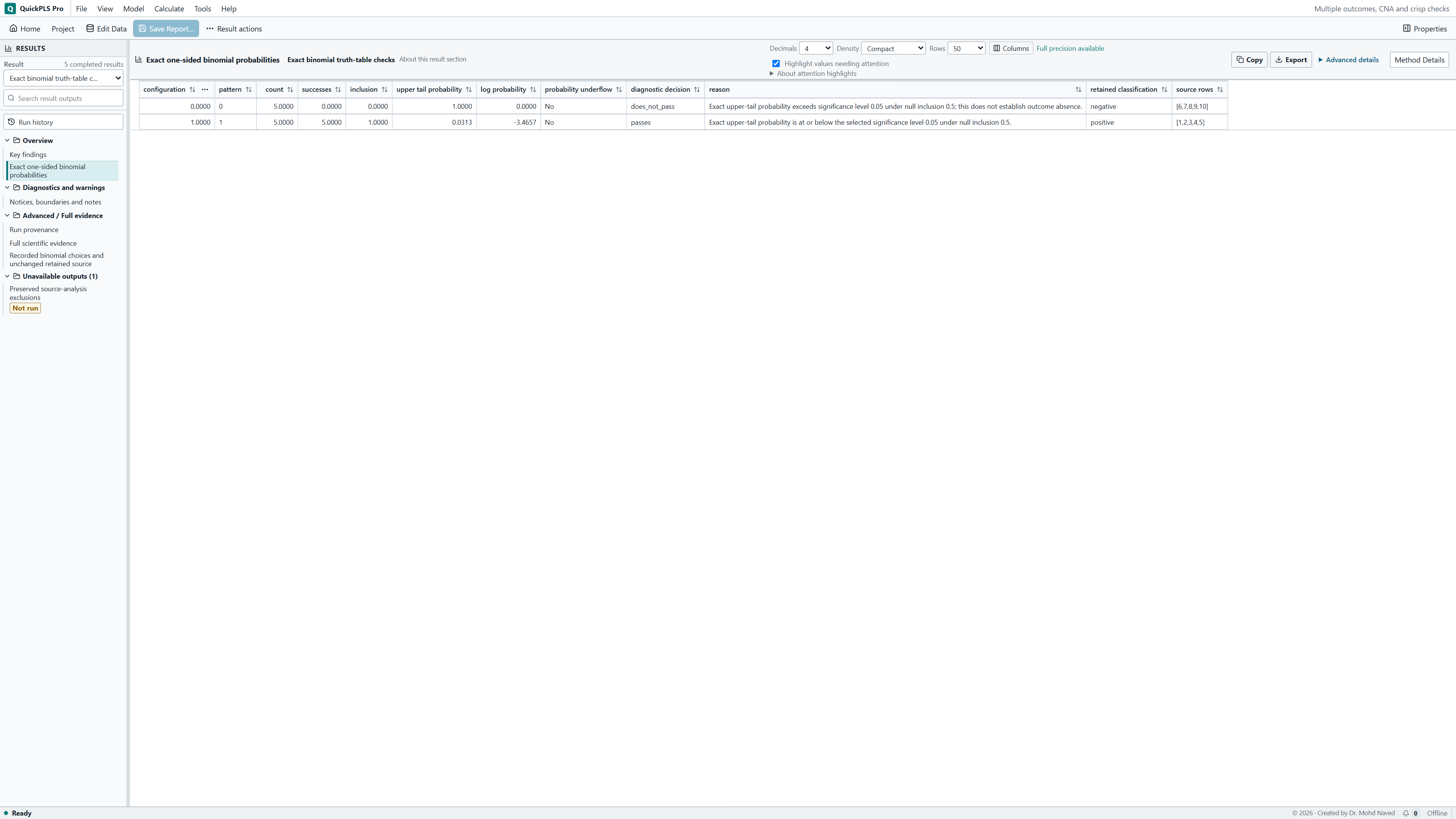
At p0=.5, five successes in five trials have an upper-tail probability of 1/32, or .03125. Upper tail means at least as many successes as the row actually contains. At alpha=.05 and minimum frequency five, the row passes both rules. Zero successes in five trials have upper-tail probability 1 because every possible count is at least zero. That result is not a lower-tail test of outcome absence.
Check that the selected source uses A alone, not A and B. With A alone this file has two five-case rows. Adding B splits those rows into groups of two or three, which changes both the counts and the upper-tail probabilities. Match the condition selection before comparing the displayed probability with the lesson.
Read successes, case count, probability and diagnostic status together. An unobserved configuration has no row probability. An observed row below the minimum frequency keeps its calculated probability but remains a diagnostic remainder, meaning it cannot qualify as positive under these diagnostic rules. The check does not adjust for testing several rows or add a second test for outcome absence. Keep the original truth table and solutions alongside it.
For a hand check at p0=.5, expect .03125 for five successes in five trials and 1 for zero successes in five trials. These are arithmetic checks against the existing teaching output, not a newly executed calculation. The app's probability decision includes equality: a value at or below alpha meets that part of the rule, provided the frequency requirement also holds.
On a small screen, swipe the table sideways to see every column.
| Output | How to read it | What to check |
|---|---|---|
| Saved crisp-calibrated result | Verify that the saved advanced-calibration result explicitly used Inclusive crisp for every selected set. | Values that happen to be 0/1 do not show that the required calibration was used. |
| Frequency n and outcome successes k | Count successes among the observed cases in this configuration. | An unobserved row has no estimated probability. A row with too few cases keeps its probability but remains a diagnostic remainder. |
| Upper-tail probability and p0 | Read the probability of at least k successes if the stated reference success probability applies. | This is a one-sided check. It has no lower-tail contradiction test or correction for testing multiple rows. |
| Alpha and row classification | Read the significance cutoff together with the minimum number of cases required. | Failure to pass does not establish outcome absence. The original truth-table classification also stays unchanged. |
Work through a row with five successes
Use crisp-outcomes.csv or a working copy of Multiple outcomes, CNA and crisp checks. Compare the saved diagnostic with the success counts you calculate by hand. Keep the original while trying different probability or frequency rules in a copy.
Set up the A-only question
Open crisp-outcomes.csv and select A as the only condition and Y as the outcome. Read A as readiness and Y as achieved delivery. The first five cases have A = 1 and Y = 1; the other five have A = 0 and Y = 0. Leave B and Z unselected for this exercise so the truth table has the intended groups.
The question is: under the stated reference probability of success, how likely would a count at least this successful be? The check adds that information to the source truth table. It does not replace the original classification rule or establish that A causes Y. Keep the probability question distinct from the study's causal explanation.
Load the explicitly crisp-calibrated source
In the sample project find Explicit crisp calibration for binomial checks. It applies Inclusive crisp thresholds of 0.5 to A and Y through Advanced calibration. Although the raw values are already zeros and ones, this explicit calibration is required by the diagnostic. Do not substitute the ordinary Existing membership result.
The saved diagnostic is Exact binomial rows: p0 0.5, alpha 0.05, frequency 5. Here p0 is the reference success probability, alpha is the probability cutoff and frequency is the minimum row case count. The names tell you what was tested. They are teaching choices, not a reason to apply the same values to every research study.
Verify the source, then inspect both rows
Find the calibrated result
Open the completed A-only, Y-outcome advanced-calibration result. Check the Inclusive crisp 0.5 thresholds for both sets and confirm all ten cases are included.
What you should see: The selected result contains eligible crisp configurations and outcome coding.
How to read it: Confirm the success event.
Load the diagnostic choices
Open fsqca_multiple_outcomes_cna.qpls and choose Data > More > Exact binomial checks. Select Explicit crisp calibration for binomial checks as the Source analysis and the saved diagnostic revision Exact binomial rows: p0 0.5, alpha 0.05, frequency 5. Choose its Owning saved study, then Load binomial choices.
What you should see: The diagnostic is linked to that completed result.
How to read it: A later change of calibration requires a corresponding calculation.
Set the three rules
Enter 0.5 under Null inclusion threshold, 0.05 under Significance level and 5 under Minimum observed frequency. Keep the explanation that these are choices for a teaching calculation.
What you should see: The three diagnostic rules, including the null probability, are explicit.
How to read it: They define the probability being computed.
Check source compatibility
Click Verify crisp source and choices and read any preparation problem. Correct the actual source type or settings; visible binary values alone do not satisfy the eligibility check.
What you should see: The source passes the crisp-data and compatibility checks.
How to read it: Fuzzy membership sums are not ordinary binomial success counts.
Preview counts and probabilities
Click Preview native binomial diagnostics. Compare each row's cases, successes, upper-tail probability, frequency eligibility and original source classification.
What you should see: The preview shows successes, trials and probabilities for the intended rows.
How to read it: Check these counts against the cases.
Save and calculate
Click Save binomial revision, then Calculate and retain binomial diagnostics. Keep the resulting diagnostic with the exact source result it examined.
What you should see: The completed result retains the null value and tail direction.
How to read it: Interpret the check as a diagnostic of those rows.
Work out the five-out-of-five result
For A = 1, all five cases have Y = 1. At p0 = 0.5, at least five successes in five trials can only mean exactly five. Its probability is 0.5 to the fifth power, or 1/32 = 0.03125. That is below alpha 0.05, and the row also meets minimum frequency 5.
For A = 0, the five cases contain zero successes. At least zero successes has probability 1, so this row does not pass the chosen upper-tail rule. That does not separately test or prove outcome absence. The hand calculations agree with the existing saved binomial output for the stated success direction.
On a small screen, swipe the table sideways to see every column.
| Condition row | Cases n | Successes k | Upper-tail probability | Meets frequency 5 | Passes alpha 0.05 |
|---|---|---|---|---|---|
| A = 1 | 5 | 5 | 0.03125 | Yes | Yes |
| A = 0 | 5 | 0 | 1 | Yes | No |
See which decision changes when a setting changes
Keep five successes out of five but change p0 to 0.6. The probability becomes 0.6 to the fifth power = 0.07776 and no longer meets alpha 0.05. Alternatively, keep p0 = 0.5 but choose alpha 0.01: the original 0.03125 no longer meets that cutoff. These arithmetic comparisons show why the reference and cutoff belong beside any reported conclusion.
Raise minimum frequency to 6 and neither five-case row can qualify as positive under the diagnostic rules, although its probability can still be calculated. Frequency asks whether the row has enough observations; the probability rule asks how unusual its successes would be under p0. A below-frequency row has not become a zero-probability row, and its cases have not disappeared.
Understand what happens when you add B
Adding B splits the same ten cases into four A/B configurations: 00 has three cases, 01 has two, 10 has three and 11 has two. The positive configurations now contain three successes out of three and two out of two. At p0 = 0.5 their upper-tail probabilities are 0.125 and 0.25.
Neither is below 0.05, and neither meets minimum frequency 5. The A-only result and these narrower rows answer different counting questions. You now have fewer observations per combination. Choose the conditions for the research question and inspect these counts before interpreting a change in diagnostic status.
Explain what the probability does and does not mean
The original calibrated analysis keeps its positive and negative row classifications. This separate result adds one exact upper-tail probability. It does not test the opposite tail, adjust automatically for checking multiple rows or replace the reasons for choosing the calibration and cases.
Explain why the reference success probability makes sense and how many rows you examined. The binomial model assumes independent trials with the same reference success probability. Repeated observations of the same organisation or closely related cases may not meet that assumption. Alpha is not the probability that a hypothesis is false, and the reported probability is not the chance that a finding will replicate. It describes a case count under the stated reference model.
Match the condition selection and row count before comparing probabilities
The matching result for this exercise must show A as the sole condition and two rows with five cases each. At p0 = 0.5, the row with five successes has probability 0.03125. A row with two successes out of two instead has probability 0.25. Both can be correct for their own counts; only the first is the intended A-only example.
When a number differs from the image, first compare the condition selection, case count and reference probability. The values 0.03125, 0.125 and 0.25 here belong to rows with different success counts. A similar-looking table can therefore be correct without showing the same probability.
Find which rule a row did not meet
Check source eligibility first, then the row's actual case count and success count. Finally read the chosen reference probability, cutoff and diagnostic status. This tells you whether a row is unsupported, below frequency or simply does not meet the stated probability rule. Changing a rule just to make the row pass would answer a new question.
On a small screen, swipe the table sideways to see every column.
| Symptom | What to check | Action |
|---|---|---|
| The source is rejected despite binary values | Whether the result explicitly used Inclusive crisp through Advanced calibration | Select or prepare the supported calibrated source. |
| The positive row shows 0.25 instead of 0.03125 | Whether B was added and the row has two cases | Compare the actual condition set and row counts. |
| A low probability is marked ineligible | The selected minimum frequency | Report whether the row meets the minimum case count separately from its probability. |
| A row changes after changing p0 | The reference success probability | Explain the new reference success probability and save a separate diagnostic revision. |
| The source solution does not change | Whether only the diagnostic was recalculated | Report the diagnostic alongside the unchanged source classification. |
| A non-passing upper-tail test is called proof of absence | The direction of the implemented test | Avoid inferring an unperformed lower-tail or absence test. |
Put counts and choices next to each probability
Report the calibrated source, selected conditions and outcome, reference probability, cutoff and minimum frequency. Show the observed count and successes for each interpreted row. Keep the diagnostic decision separate from the original truth-table classification so readers can see exactly what the additional calculation contributed.
| Item | Teaching value |
|---|---|
| Source calibration | Inclusive crisp 0.5 for A and Y |
| Reference probability; alpha; frequency | 0.5; 0.05; 5 |
| A-positive count | 5 successes in 5 cases |
| A-positive upper-tail probability | 0.03125 |
| A-negative upper-tail probability | 1 |
| Numerical origin | Hand binomial arithmetic and existing saved diagnostic |
Example Methods paragraph
We applied the exact upper-tail binomial diagnostic to a saved advanced-calibration result with Inclusive crisp for both the A condition and Y outcome. The teaching choices were reference probability 0.5, alpha 0.05 and minimum frequency 5. We reported row counts and whether each row met the diagnostic rules separately from the source truth-table classifications.
Explain the row before explaining its probability
A suitable Results account would say that the A-positive row had five successes in five cases and upper-tail probability 0.03125 at p0 = 0.5. It met frequency 5 and alpha 0.05. The A-negative row had no successes in five cases and probability 1. These separate checks left the original truth-table classifications unchanged.
- Calculate 0.5 to the fifth power and connect it to the five successes.
- Show how selecting B splits the original rows into smaller groups.
- Explain the frequency rule separately from the probability cutoff.
- State that the test counts results at least as successful in the selected outcome direction.
- Identify the actual crisp-calibrated source and the saved diagnostic choices in the report.
Keep the probability check beside the original solution
The diagnostic does not change the source truth-table classifications or rerun their minimization. It supplies one upper-tail check, without a lower-tail test or adjustment for multiple row tests. Use the required Inclusive crisp source so the saved result records how every selected set became binary.