 QuickPLS
What the method does
Partial least squares structural equation modelling (PLS-SEM) represents each construct by a weighted combination of its indicators, then estimates the relationships drawn between constructs. The measurement model specifies which indicators belong to each construct and whether they reflect or form it. The structural model specifies the proposed relationships. Estimation produces weights, loadings, path coefficients and explained variance; measurement assessment and uncertainty are separate parts of interpreting those estimates.
Construct score: zⱼ = Σₖ wⱼₖxⱼₖ. Structural equation: zⱼ = Σₕ βⱼₕzₕ + εⱼ.
For one case, xⱼₖ is indicator k of construct j and wⱼₖ is its weight. The weighted sum gives the construct score zⱼ. A path coefficient βⱼₕ describes the relationship from a predictor score zₕ to zⱼ, with the other predictors in that equation held constant; εⱼ is the residual. The PLS algorithm updates the weights until its stopping criterion is met. A path coefficient alone does not establish causation.
Data and analysis in QuickPLS
Use a case-by-variable table: one respondent or other observational unit per row and numeric indicators in columns. Define the indicator direction, missing-value codes and reflective or formative blocks before estimation. Sample size should follow the study design and effects of interest.
QuickPLS lets you import your own suitable dataset, draw the measurement blocks and paths, run PLS-SEM, inspect the results and export a report. The example below teaches that workflow; its construct names and data are not required for your own analysis.
Follow a worked example
The following example shows the data, settings and decisions for one analysis. Use the linked practice files to follow it. For your own study, keep the procedure and choose the variables, model and settings that fit your research question.
Download customer-experience.csv to begin. It contains 240 rows and 13 columns. The example below identifies the variables to use, their roles and any rows to exclude; not every column is an analysis variable.
The study and model
This example asks how service quality and trust relate to customer satisfaction, and how satisfaction relates to loyalty. Each concept is measured by several survey indicators. Partial least squares structural equation modelling (PLS-SEM) forms construct scores from these indicators and estimates the specified relationships between the scores.
The exercise uses synthetic data. It provides a complete model specification and checked point estimates, followed by measurement assessment, bootstrap inference and reporting. A point estimate is the fitted value before a confidence interval is added. Complete this analysis before attempting the optional extensions.
| Term | Meaning in this example |
|---|---|
| Construct | An idea you want to study, such as Trust or Satisfaction. |
| Indicator | A measured column used to represent an idea. trust_1, trust_2 and trust_3 are the three indicators of Trust. |
| Construct score | A value formed from a construct's indicators for each case. |
| Path | A proposed relationship drawn as an arrow between constructs, such as Trust → Satisfaction. |
| Case | One row in your data. A real customer study would normally have one respondent per row. |
Project preparation
Create a writable QuickPLS project named First customer study. The project keeps the imported data, model and saved calculations together. Use the supplied file for the initial analysis so that your results can be compared with the answers below.
For a real survey, document what each question measures, its response scale and any reverse coding before drawing the model. The reflective measurement choices in this exercise are part of its teaching specification; they do not establish that your own instrument has the same structure.
1. Import the data
Download customer-experience.csv. It contains 240 synthetic cases, twelve numeric measurement columns and case_id, which identifies each row. The four indicator blocks are listed below. Do not assign case_id to a construct.
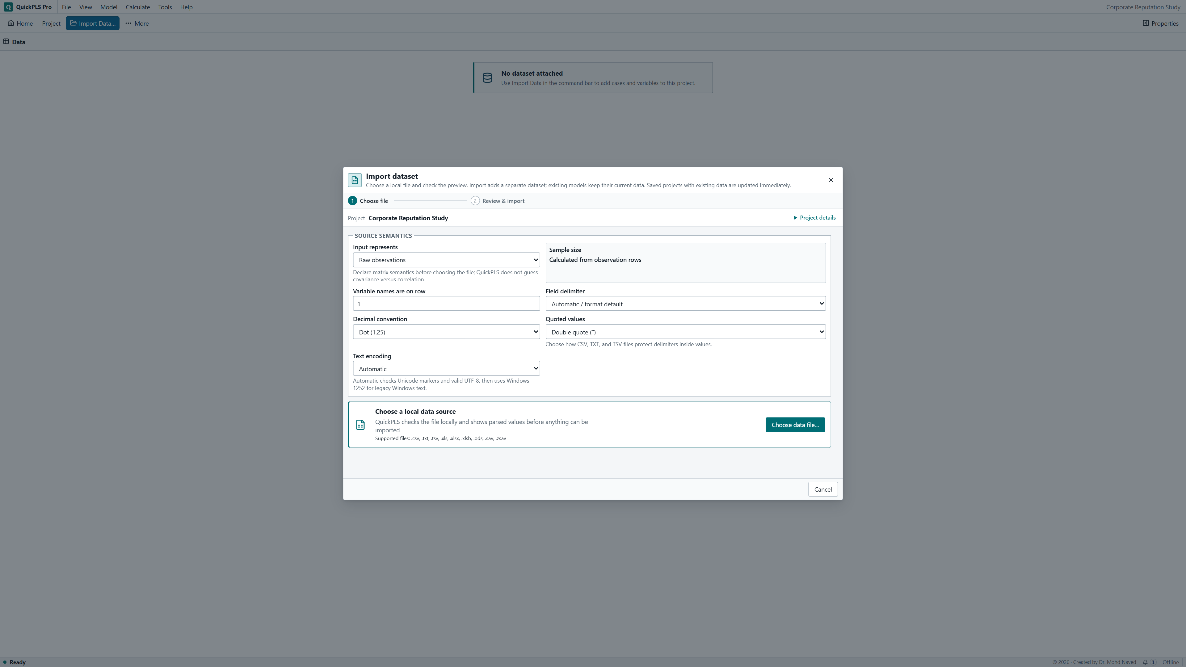
In the writable project, choose File → Import Data… (Ctrl+I), then Choose data file…. Select the CSV. In Review & import, check raw-data input, Header row 1, comma separator and Decimal convention Dot (1.25). Treat the twelve measurement columns as Continuous. Click Import dataset and confirm Dataset imported and verified, then check that the imported dataset has 240 cases.
Before creating the model, inspect the imported column names and 240-case count. The customer file contains only the twelve measurement columns and case_id; the separate workshop exercises use a different file.
On a small screen, swipe the table sideways to see every column.
| Construct to create | Assign these three indicators | Measurement for this exercise |
|---|---|---|
| Quality | quality_1, quality_2, quality_3 | Reflective |
| Trust | trust_1, trust_2, trust_3 | Reflective |
| Satisfaction | satisfaction_1, satisfaction_2, satisfaction_3 | Reflective |
| Loyalty | loyalty_1, loyalty_2, loyalty_3 | Reflective |
2. Specify the measurement blocks and paths
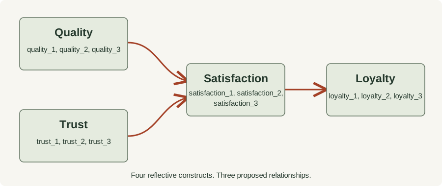
All four constructs use reflective measurement: their indicators are treated as expressions of the corresponding concept. Satisfaction has two predictors, Quality and Trust; Loyalty has one predictor, Satisfaction. The baseline model has no direct Quality → Loyalty or Trust → Loyalty path.
Create the model
Choose File → New Model…. Name it Customer experience, select the imported customer-experience Dataset version and confirm Cases shows 240. Click Create model.
What you should see: A model named Customer experience is linked to the 240-case dataset.
How to read it: Correct the dataset selection before assigning indicators.
Create Quality
Open Indicators. Select quality_1, then hold Ctrl while selecting quality_2 and quality_3. Confirm 3 selected and click Create construct.
What you should see: Quality has three assigned indicators.
How to read it: A selected column is not assigned until Create construct has been used.
Name the construct
Choose Select and click the construct body. If needed, open View → Show Properties. In Properties → Model, enter Quality in Name and press Enter.
What you should see: The construct label reads Quality.
How to read it: Press Enter to commit the name before moving to the next construct.
Set its measurement role
In Properties → Parameter, set Measurement model to Reflective.
What you should see: The Properties panel shows Reflective.
How to read it: This is the teaching model’s measurement assumption; use theory to choose the role in your own study.
Create the remaining blocks
Repeat for Trust, Satisfaction and Loyalty using their three matching indicators in the table. Give each construct its stated name and select Reflective. Each indicator belongs to one block.
What you should see: There are four constructs, each with its own three indicators.
How to read it: Remove any duplicated or misplaced assignment before adding paths.
Connect the constructs
Choose Connect. Drag from the body of Quality to Satisfaction, from Trust to Satisfaction, and from Satisfaction to Loyalty. Check each arrow direction, then return to Select.
What you should see: Quality and Trust point to Satisfaction; Satisfaction points to Loyalty.
How to read it: A reversed arrow specifies a different equation.
Check and save
Confirm four constructs, three indicators per construct and the three specified paths. For a missing assignment, select the construct and column, then choose Assign to [construct name]. Remove an incorrect assignment through Properties → Data Binding → Remove. Save the model.
What you should see: The model has four blocks and exactly three baseline paths.
How to read it: Save this specification before opening Calculate.
3. Estimate the model
Click Calculate… on the model toolbar. In Find a method, select PLS-SEM Algorithm; open Methods if the list is collapsed. Use the controls below. Casewise deletion excludes a case with a missing required indicator, but this complete practice file retains all 240 cases.
Review the selected inputs
Check Readiness, the Customer experience model and the customer-experience dataset. Resolve any setup problem identified by the app.
What you should see: Readiness identifies the Customer experience model and the imported 240-case file.
How to read it: Resolve a different selection or an incomplete model before starting.
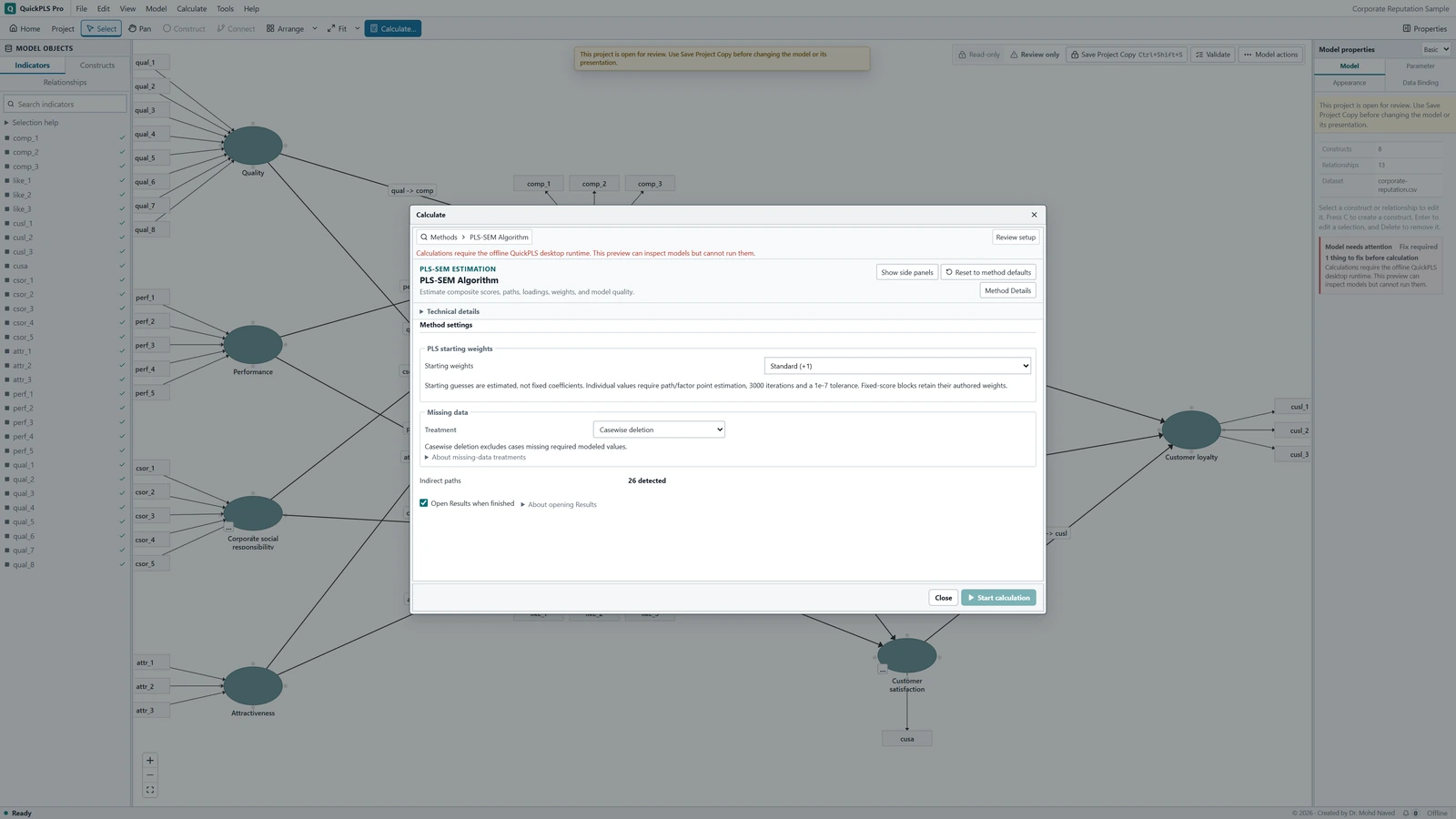
PLS-SEM Algorithm settings in QuickPLS. Select your own dataset and model, then use the choices described in the steps. Run the calculation
Keep Open Results when finished selected and click Start calculation. If prompted, save the project or a writable copy and continue.
What you should see: A new completed calculation opens in Results.
How to read it: Keep that result selected while reading its tables; a different saved calculation can have different settings.
Confirm convergence
Check that the calculation converged: its repeated estimation steps settled within the stopping criterion. Investigate a convergence message before interpreting the estimates.
What you should see: The estimation summary reports convergence and 240 analysed cases for this complete file.
How to read it: If either differs, check the imported data and calculation status before comparing the answer table.

On a small screen, swipe the table sideways to see every column.
| Control | Choose | What it does |
|---|---|---|
| Starting weights | Standard (+1) | Uses the standard initial weights for the calculation. |
| Missing data → Treatment | Casewise deletion | Uses rows with values for every required indicator. This practice file is complete. |
Recorded calculation settings
These settings record how the checked answers were calculated using the QuickPLS calculation code outside the desktop app. Path weighting, the iteration limit and the stopping criterion describe that calculation; they are not additional editable fields in this ordinary raw-data dialog.
On a small screen, swipe the table sideways to see every column.
| Setting | Use for this exercise | Why it is recorded |
|---|---|---|
| Method | Ordinary PLS-SEM | Keeps this exercise separate from consistent PLS and other estimators. |
| Measurement blocks | Four reflective blocks, Mode A updates | Matches the checked definition of the four constructs. |
| Weighting scheme | Path | Specifies how relationships contribute to the PLS calculation. |
| Data scale | Standardised | Puts the indicators on a common scale. |
| Missing-data treatment | Listwise deletion; shown as Casewise deletion in the example screen | Excludes a row if a required model value is missing. All 240 cases are complete in this file. |
| Maximum iterations | 3,000 | Limits the repeated estimation steps. |
| Stopping criterion | 0.0000001 | Sets the convergence tolerance. |
| Bootstrap samples for this first comparison | 0 | The answer check below concerns the estimates themselves. Uncertainty is a separate step. |
4. Locate the results
In Results, select the completed calculation from the Result dropdown. Open the folders listed below, or enter an output name in Search result outputs. Clear the search to restore the full list. Choose Table where Table and Visual tabs are available.
Graphical Output provides an overview: arrows carry path coefficients, indicator values are loadings, and R² is shown for outcomes with incoming paths. Use the named tables for reporting so that each value remains attached to its construct, indicator or relationship.
Keep Customer experience selected in the Result dropdown while checking the tables. Match construct and indicator names before comparing the values with the answer table below.
On a small screen, swipe the table sideways to see every column.
| What you need | Open this folder and output | What to read |
|---|---|---|
| Model picture with paths, loadings and R² | Overview → Graphical Output | Use the diagram as an overview, then read the named tables. |
| Indicator loadings | Estimates → Outer loadings | Find each construct and indicator row. Use this table for the strength and direction of an indicator's relationship with its construct. |
| Path estimates for the three drawn arrows | Effects → Direct effects | Read the source and destination construct together. Match Quality → Satisfaction, Trust → Satisfaction, and Satisfaction → Loyalty before comparing numbers. |
| Explained variation | Estimates → R-squared | Read the Satisfaction and Loyalty rows. Search R-square if the output title uses R-square rather than R-squared. |
| Reliability and average variance extracted | Reliability and validity → Construct reliability and validity | Read one construct across the row. Do not confuse rho_A and composite reliability, and do not report AVE as a reliability coefficient. |
| Whether reflective concepts are distinguishable | Discriminant validity → HTMT+ | Read each eligible pair of reflective constructs. All four constructs in this customer model are reflective; inspect the pair names before interpreting their HTMT+ values. |
| Overlap among predictors of the same outcome | Collinearity and effects → Inner VIF values | Read predictor and outcome together. The two predictors of Satisfaction are examined within the Satisfaction equation. |
| Contribution of each predictor | Collinearity and effects → f-square effect sizes | This describes how much explained variation changes when a predictor is removed from that equation. It is different from the path coefficient and its p-value. |
| Explained variation with predictor-count adjustment | Model fit → R-square and adjusted R-square | Keep R-square and adjusted R-square separate in your report. This table's placement does not make R-square a global model-fit test. |

5. Check the point estimates
Match the named paths and outcomes before comparing values. For the same data and specification, the three path coefficients and two R² values should agree with the six-decimal answers below.
The answer pack compares QuickPLS calculations performed outside the desktop app with an independent cSEM calculation in R. It checks 29 values: three paths, twelve loadings, twelve weights and two R² values. These are point estimates; the pack does not supply checked confidence intervals or p-values.
| Result | Expected value, rounded |
|---|---|
| Quality → Satisfaction | 0.444622 |
| Trust → Satisfaction | 0.431074 |
| Satisfaction → Loyalty | 0.646988 |
| Satisfaction R² | 0.491364 |
| Loyalty R² | 0.418593 |
Complete measurement answers and calculation record
The loadings and weights below are rounded to six decimal places from the same customer-experience calculation. A loading describes the association between an indicator and its construct score; a weight is a coefficient used to form that score. They are different quantities.
On 6 November 2026, QuickPLS calculation code was run outside the desktop app. It converged in 5 iterations and used all 240 cases. The answer pack records the software and settings; this check did not rerun the Microsoft Store app.
The independent check used R 4.6.1 and cSEM 0.7.1. All 29 absolute differences were below 0.00000001; the largest was 1.2212453270876722e-15. The archive includes the input CSV, expected output, settings and reference calculation. Its settings file is a readable record, not an importable QuickPLS project.
This check does not include bootstrap inference or a complete assessment of reliability and validity. Inspect those outputs in the relevant saved calculation before writing a substantive research conclusion.
On a small screen, swipe the table sideways to see every column.
| Indicator | Loading, rounded | Weight, rounded |
|---|---|---|
| quality_1 | 0.928120 | 0.363112 |
| quality_2 | 0.924467 | 0.345072 |
| quality_3 | 0.931147 | 0.369416 |
| trust_1 | 0.923406 | 0.366507 |
| trust_2 | 0.919423 | 0.352480 |
| trust_3 | 0.908457 | 0.371495 |
| satisfaction_1 | 0.925546 | 0.363315 |
| satisfaction_2 | 0.937055 | 0.371487 |
| satisfaction_3 | 0.922492 | 0.342151 |
| loyalty_1 | 0.932123 | 0.359873 |
| loyalty_2 | 0.934764 | 0.353169 |
| loyalty_3 | 0.936855 | 0.356966 |
6. Assess the measurement model
Interpret the structural paths only after examining what their constructs measure. For each reflective block, begin with indicator direction and content, then assess reliability and average variance extracted (AVE). Reliability concerns consistency among indicators; AVE summarises the indicator variance represented by the reflective construct.
Discriminant validity concerns whether constructs intended to represent different concepts can be distinguished. The heterotrait-monotrait ratio, HTMT, compares relationships between indicators of different constructs with relationships within each construct. Inspect each eligible pair, including Quality and Trust, alongside the item wording. High reliability within two blocks does not establish that the blocks measure different concepts.
Formative measurement requires a different assessment. Its indicators define the composite, so their content, weights and collinearity matter. Collinearity is overlap among indicators that can make their separate contributions unstable. Reflective reliability and AVE do not assess whether a formative composite covers its intended content.


Interpret loadings, weights and validity checks
The checked loadings and weights appear with the answer table above. Read a loading as an indicator’s association with the construct score, not its contribution to a structural path. Check the sign against the question’s coding. A negative loading may reflect a reverse-worded item, a coding error or a measurement problem.
For an arithmetic illustration, suppose three standardised loadings are 0.80, 0.70 and 0.90. Their AVE is (0.64 + 0.49 + 0.81) / 3 = 0.6467. These hypothetical values explain the calculation; they are not the fitted loadings or AVE for either practice dataset.
Use the table below to organise the assessment. State the criteria appropriate to the instrument and field. If an item performs poorly, inspect its meaning and coding before considering removal. An item can cover content that the others omit; deleting it may improve a statistic while narrowing the construct. Save any justified alternative as a separate model and explain the change.
On a small screen, swipe the table sideways to see every column.
| Output | Example or check | How to respond |
|---|---|---|
| Outer loadings | Illustrative values: 0.80, 0.70 and 0.90 | Read direction, item wording and the rest of the block together. |
| Outer weights | Each indicator's contribution to forming the score | For formative measurement, examine contribution, uncertainty and content coverage; do not substitute loading rules. |
| Reliability and AVE | Illustrative AVE: 0.6467 | Use for the reflective blocks to which these measures apply. |
| HTMT | Check each eligible pair and any available uncertainty result | If two constructs overlap, inspect their definitions and similar item wording before changing the model. |
| VIF | Variance inflation factor at the indicator or predictor level shown | A large value signals overlap that can make separate contributions unstable. Inspect which variables share information. |
| Descriptive fit | SRMR, d_ULS or d_G for the stated model representation | These summarise discrepancies between the model and observed relationships in different ways. A point value is not automatically a bootstrap test of exact fit. |
7. Interpret the structural relationships
Quality → Satisfaction is 0.444622 and Trust → Satisfaction is 0.431074. Each coefficient is estimated while accounting for the other predictor in the Satisfaction equation. They are adjusted relationships in one model, not two separate correlations.
The scores are standardised. Holding Trust constant, a difference of one standard deviation in Quality corresponds to about 0.445 standard deviations in fitted Satisfaction. This is not a 44.5% increase in satisfaction. Satisfaction → Loyalty is 0.646988; Satisfaction is the only predictor of Loyalty in this baseline model.
Satisfaction R² is 0.491364 and Loyalty R² is 0.418593. The fitted model therefore accounts for about 49.1% and 41.9% of the variation in these scores. R² describes the analysed sample. Evidence about prediction for new cases requires a separate prediction assessment.
The two Satisfaction coefficients are close. Their point estimates alone do not establish that Quality has a larger relationship than Trust. Assess a claimed difference directly, and interpret each estimate with its uncertainty and practical meaning.
Hypothetical example
Separate arithmetic example
If a different model had Quality → Satisfaction = 0.40, Trust → Satisfaction = 0.20 and Satisfaction R² = 0.45, the last value would mean 45% of the fitted Satisfaction variation. These invented numbers explain the interpretation; they are not the answers for customer-experience.csv.
8. Estimate uncertainty with bootstrapping
Bootstrapping repeatedly samples whole cases with replacement and refits the model. Variation across these refits is used to estimate uncertainty. Keeping each sampled case intact preserves the relationships among its indicators.
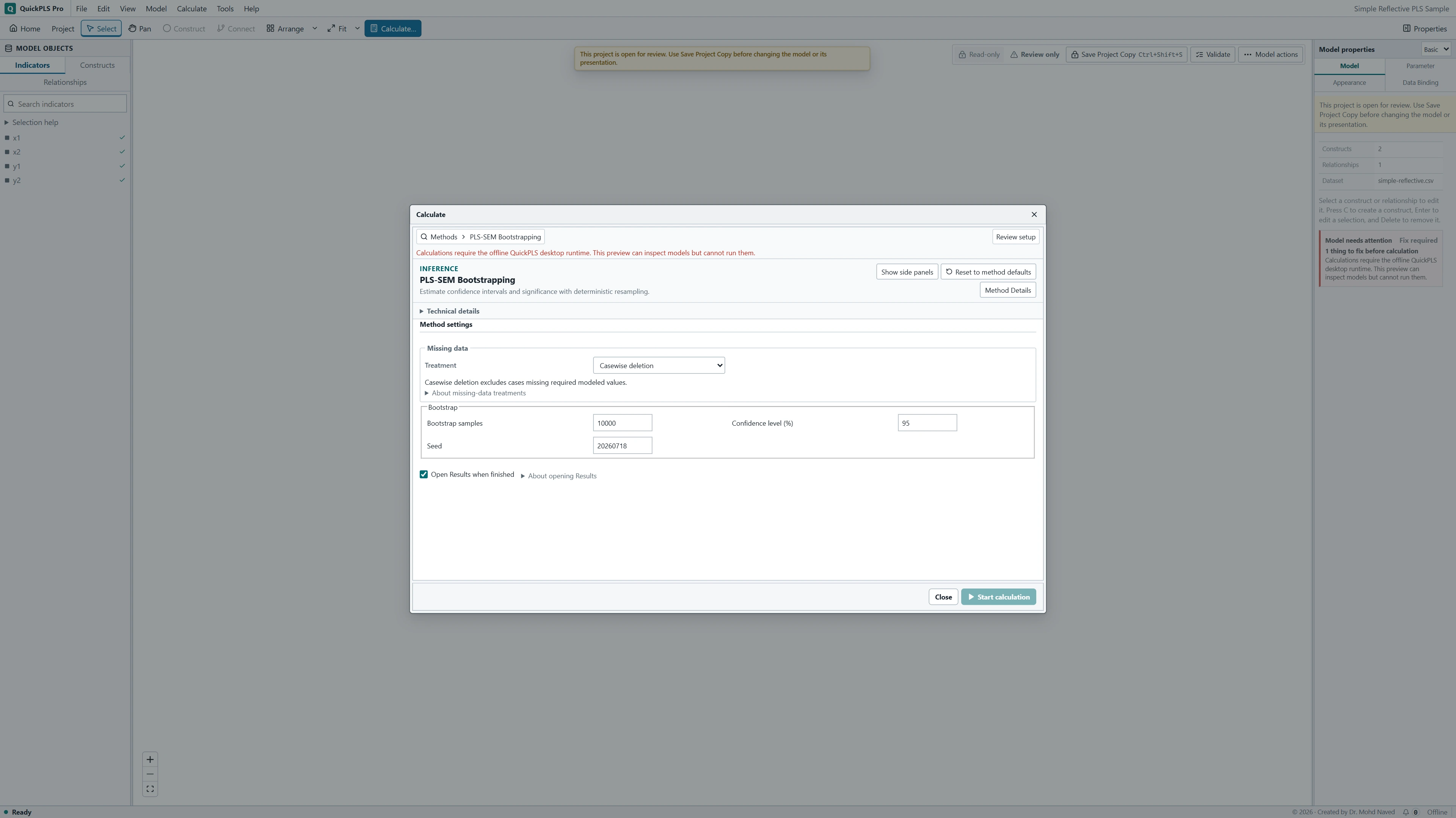
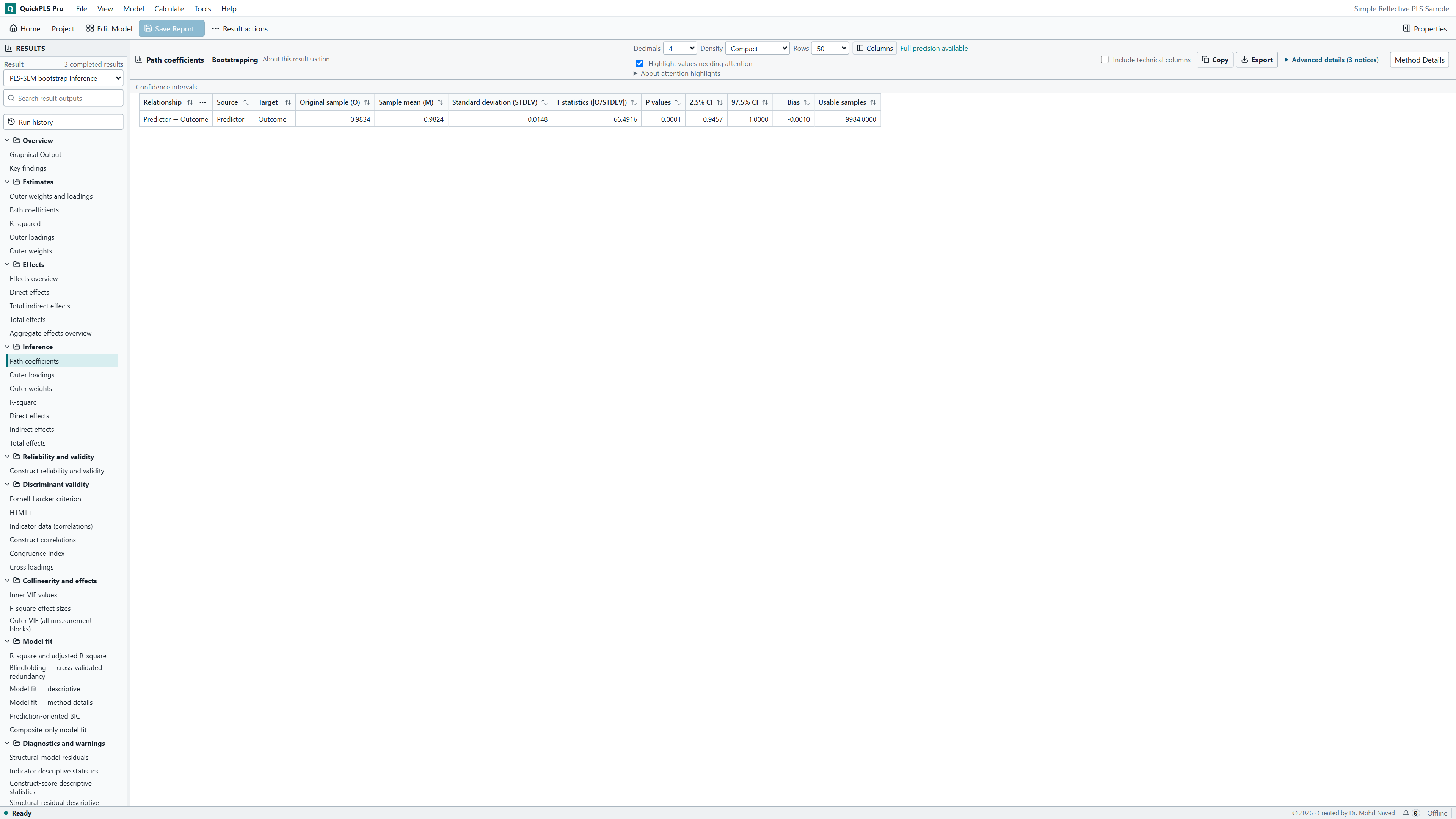
For the same saved model and dataset, open Calculate and select PLS-SEM Bootstrapping. As a teaching run, enter 1,000 Bootstrap samples, Confidence level (%) 95 and Seed 20261105. The seed supports repeatability of the random draws with the same setup. These choices follow the separate bootstrap lesson; this page does not provide checked answers for that run.
Read the interval method named in the output and the requested, usable and failed resample counts. Investigate failures, including constant indicators or convergence problems, before relying on the intervals. Report the method and usable count with the estimates.
An interval spanning zero does not clearly distinguish a positive from a negative relationship at the stated confidence level. An interval entirely above zero supports a positive relationship under the analysis assumptions. In both cases, consider the range of plausible effect sizes rather than treating significance as the substantive result.
After calculation, select the new bootstrap result and locate each named effect with its matching interval. Keep the point-estimate result available for comparison, but use the bootstrap result’s own settings and usable-refit count when reporting uncertainty.
Interpretation of an association
A positive Quality → Satisfaction coefficient describes the association after accounting for the specified Trust path. It does not establish that an intervention improving quality would cause the estimated change in satisfaction. That conclusion requires support from the study design and its assumptions.
Diagnose unexpected results
First distinguish a specification or coding error from a substantive finding. Use the checks below, preserving the original result so that any correction can be traced to a changed input or model.
If the intended model and data are correct, a small estimate or wide interval is a result to explain. Revise the model only for a defensible measurement or research reason, and report the effect of that revision.
On a small screen, swipe the table sideways to see every column.
| What you notice | Check first | A useful next step |
|---|---|---|
| Your five practice answers differ | The file, 240-case count, three arrows, indicator assignments and settings | Match the stated exercise. Keep any deliberately different model separate. |
| A loading has an unexpected sign | The item wording, reverse coding and direction of the construct score | Correct a genuine coding error using the data documentation. Keep the correction in your notes. |
| One reflective indicator has a weak loading | Whether it measures the intended idea and whether the item was coded correctly | Assess its content alongside the other indicators. Save a justified alternative model rather than removing items until a threshold is passed. |
| Reliability is high but constructs overlap | HTMT results, similar wording and whether the concepts are truly different | Review the construct definitions. High reliability alone does not establish that the two concepts are distinct. |
| A formative weight is small or unstable | Overlap between indicators, VIF and what each indicator contributes | Consider uncertainty and content coverage before dropping a component. |
| A path is small or its interval crosses zero | The direction, uncertainty, sample and originally stated question | Explain the estimate and the range it allows. More data may improve precision, but cannot guarantee the relationship you expected. |
| R² is lower than expected | Which outcome it belongs to and whether the model matches the research question | Discuss the amount explained in context. Add predictors only when the research argument supports them. |
| Bootstrapping reports failed resamples | The failure messages, constant indicators, estimation problems and convergence | Investigate the affected fits and report usable and failed counts with the intervals. |
| An indirect effect differs from hand multiplication | The specific path, coefficient scale and saved model | Multiply the correct paths from the same model. Use the indirect effect's own interval. |
| A higher-order choice is unavailable | The measurement roles, position in the model and selected approach | Choose a supported approach that still represents the intended concept, and explain any change. |
| Results change after handling missing values | Which cases were included and how original variables and generated terms were prepared | Compare the actual inputs and preparation steps. Keep both analyses if they answer a useful sensitivity question. |
9. Save the analysis
Select the completed result, use Save Report and export the required tables or figures. Reopen the project and report to confirm that they refer to the same calculation.
Keep the data version, analysed case count, indicator assignments, paths and calculation settings with the output. Save revised specifications separately. The reporting table below identifies what a reader needs to reproduce and assess the analysis.
Methods and results wording
Methods for the checked example: We fitted a PLS-SEM model to 240 synthetic cases. Quality, Trust, Satisfaction and Loyalty were specified as reflective constructs with three indicators each. The structural paths were Quality → Satisfaction, Trust → Satisfaction and Satisfaction → Loyalty. Estimation used path weighting, standardised data, listwise deletion, a maximum of 3,000 iterations and a stopping criterion of 0.0000001.
Results for the checked example: Quality and Trust were positively associated with Satisfaction, with standardised coefficients of 0.444622 and 0.431074. The Satisfaction → Loyalty coefficient was 0.646988. The model accounted for approximately 49.1% of the fitted variation in Satisfaction and 41.9% in Loyalty. These are point estimates from the synthetic practice data.
A research report must also present the relevant measurement assessment and any inference actually completed. Add the confidence interval for each reported effect, its method and confidence level, the bootstrap count and seed, and the usable and failed refit counts. The point estimates above do not establish statistical significance.
For a weak or imprecise result, suitable wording is: The estimated relationship was small, and its interval included values on either side of zero. Supply the actual estimate and interval bounds with that sentence, then explain which substantive interpretations remain compatible with the result.
| Report section | Include |
|---|---|
| Data | The source, actual analysed count, indicator meanings and missing-data decisions. |
| Measurement | Reflective or formative roles, the relevant loadings or weights, and suitable reliability and validity checks. |
| Structure | The named paths, score scale, estimates, matching confidence intervals and each outcome's R². |
| Extensions | The exact indirect path, interaction construction or higher-order stages, if used. |
| Computation | Weighting, scaling, convergence and the corresponding resampling settings and counts. |
| Interpretation | The study-design assumptions, useful sensitivity checks and any separate prediction results. |
Practice review
Reopen your saved analysis and locate the five checked structural values. Use the tasks below to check whether you can explain the model as well as reproduce its numbers.
- Identify the four constructs and their three indicators. Distinguish a loading, a weight and a path coefficient using a row from the corresponding table.
- Interpret one R² value without calling it prediction accuracy. Calculate the hypothetical AVE and explain why it is not an answer from the fitted practice model.
- Explain an interval that includes zero in terms of effect size and uncertainty. Identify the measurement evidence needed before interpreting the structural paths.
- If completing an extension, identify its indirect route, moderator values or higher-order stages. For matrix or incomplete data, explain which observations and preparation choices the result depends on.
Scope of the example
The synthetic customer data demonstrate estimation and interpretation; they provide no empirical evidence about customers. The checked answer pack verifies the stated numerical calculation, not the validity of a questionnaire or the adequacy of a research design.
For your own study, justify the measurement structure and paths from the research question. Causal claims require design and identification assumptions, while claims about new-case prediction require a prediction assessment. Neither follows from reproducing the point estimates in this tutorial.
Optional methods and settings
Mediation: an indirect pathway through Satisfaction
The route Quality → Satisfaction → Loyalty represents a specific indirect effect. To assess it alongside the direct Quality → Loyalty relationship, copy the baseline customer model and add that direct path. Retain the original indicator blocks and the other paths. The resulting estimates belong to this extended model, not to the baseline answer table.
The separate research-workshop.csv offers an alternative 360-case synthetic exercise. If using it, rebuild Quality, Trust, Satisfaction and Loyalty from their _1, _2 and _3 indicators, with the original three paths before adding the direct path. Exclude case_id, group, weight and the supplied arithmetic means from the indicator blocks. Keep this dataset and its results separate from the 240-case customer exercise.
Estimate and report the indirect effect
In a linear model without an interaction, the specific indirect effect is the product of the paths along its route. For a hypothetical Quality → Satisfaction coefficient of 0.50 and Satisfaction → Loyalty coefficient of 0.40, the product is 0.50 × 0.40 = 0.20. If Quality → Loyalty is 0.10, the corresponding total effect is 0.30. These values illustrate the calculation; they are not fitted answers for either download.
Bootstrap the complete model to estimate uncertainty in the indirect effect. Each resample re-estimates the paths and their product together. Multiplying the endpoints of separate path intervals does not yield an interval for the product.
Where several indirect routes exist, report the specific effects before their sum. Positive and negative routes can offset one another, so a small total indirect effect need not mean that every route is small.
Save the extended specification
In a separate model, add Quality → Loyalty and identify Quality → Satisfaction → Loyalty as the indirect route to assess.
What you should see: The saved model includes the added Quality to Loyalty path and the route through Satisfaction.
How to read it: Retain the baseline model so the extended specification remains identifiable.
Estimate and bootstrap
Run PLS-SEM Algorithm and the matching PLS-SEM Bootstrapping calculation for this model and dataset.
What you should see: The extended model has its own point result and matching bootstrap result.
How to read it: Use the same model and cases for both calculations.
Match effects and intervals
Read direct, specific indirect, total indirect and total effects from the same result. Keep each confidence interval attached to its named effect and bootstrap calculation.
What you should see: The indirect route has a named estimate and its own confidence interval.
How to read it: Interpret that interval; the significance of the two constituent paths is not a substitute for it.
Moderation: a Quality relationship that depends on Trust
Moderation asks whether the Quality → Satisfaction relationship changes with Trust. An interaction between Quality and Trust represents that change. Retain both Quality → Satisfaction and Trust → Satisfaction as main effects.
With standardised moderator scores, Trust = 0 is the score mean, while -1 and 1 represent one standard deviation below and above it. The Quality main coefficient is its slope at Trust = 0, rather than a single slope applying at every Trust value. Choose moderator values that are meaningful and supported by the observed scores.
Specify the interaction and interpret simple slopes
For a hypothetical Quality main coefficient of 0.30 and interaction coefficient of 0.15, the Quality slope is 0.30 + 0.15 × Trust. It equals 0.15 at Trust = -1, 0.30 at Trust = 0 and 0.45 at Trust = 1. This arithmetic illustrates interpretation; it is not a calculated result for either practice dataset.
The ordinary Simple slope analysis table reports the Relationship, Moderator, Moderator score and Conditional effect. These are point slopes at the stated moderator values. Read uncertainty for the interaction in its matching bootstrap output; this table does not supply a separate confidence interval for each simple slope.
A difference between a significant slope and a nonsignificant slope is not itself a test that the slopes differ. A three-way interaction introduces a second moderator and requires the corresponding main effects and lower-order interactions; its conditional relationships need interpretation beyond the three-way coefficient. The linked conditional-process guide treats the related extension in more detail.
The diagram anchor marks the relationship being moderated. It is not an additional observed indicator.
Create a separate moderation model
Copy the baseline model. Choose Model → Moderating Effect…; the command may display Moderating Effect (Creates Model Revision)…. Select Quality → Satisfaction under Relationship and Trust under Moderator.
What you should see: The preparation names Quality to Satisfaction as the relationship and Trust as the moderator.
How to read it: Correct the roles before creating the revised model.
Specify the interaction construction
Under Construction, choose Two-stage, then Add moderating effect. Retain the Quality and Trust main-effect paths into Satisfaction. Check the resulting model before calculation.
What you should see: The revised model retains both main effects and adds the intended two-stage interaction.
How to read it: A missing main effect changes the meaning of the interaction equation.
Estimate and interpret
Run the revised PLS model and its matching full-model bootstrap. Report the interaction coefficient with its own interval, then use Simple slope analysis to explain the point slopes at the stated Trust scores. Keep the score scale and interaction construction with the result.
What you should see: The result separates the interaction coefficient, its interval and the conditional slopes.
How to read it: Explain how the Quality slope varies with Trust over a meaningful range of Trust scores.
Higher-order measurement: Resources, Support and Capability
A higher-order construct represents a broader concept through lower-order dimensions. This exercise defines Readiness through Resources, Support and Capability. Each dimension has reflective indicators, while the dimensions form Readiness. Reversing that relationship would make a different measurement claim.
Use the 360-case research-workshop.csv, which includes three matching indicators for each dimension and the Satisfaction block. Its definitions and data are synthetic. It is a different exercise from the 240-case customer model.
Repeated, extended-repeated, embedded and disjoint approaches differ in the indicators or scores used for estimation. Their availability depends on measurement roles and model position. The worked setup below uses disjoint two-stage estimation; it does not treat these approaches as interchangeable.
Specify a disjoint two-stage Readiness model
Create Resources, Support and Capability from their corresponding three-indicator reflective blocks, and create Satisfaction. Select all three dimensions. The wizard requires at least two eligible ordinary constructs. Open Higher-Order Construct from Model or the selection context menu.
Name the construct Readiness and choose Dimensions form the HOC. HOC means higher-order construct. Review the derived type, then open Advanced → Construction approach and select Disjoint two-stage. If Initial model path appears, choose Direction HOC → construct and Construct Satisfaction. Click Create. Check that the resulting model contains Readiness → Satisfaction; do not add the same arrow again if the wizard created it.
The first stage estimates the dimension scores. These scores become indicators in the second stage. Inspect the stage mapping so that you know which inputs produced the higher-order estimates. Embedded two-stage and repeated-indicator approaches prepare different models.
Use the output sequence below: dimension measurement, higher-order measurement, then the specified structural relationship. Distinguish the research path Readiness → Satisfaction from any paths generated to perform the estimation.
For uncertainty, use the supported full-model higher-order bootstrap, which refits the required stages from the original cases. Check the effects and interval methods available for this specification. Bias-corrected and accelerated (BCa) intervals use a bias adjustment and leave-one-case-out calculations; studentized intervals use additional resampling. Neither is available for every higher-order target.
On a small screen, swipe the table sideways to see every column.
| Output | Question it answers | Check |
|---|---|---|
| Dimension measurement | Do Resources, Support and Capability have suitable indicators? | Assess each original indicator block. |
| Higher-order weights or loadings | How does Readiness relate to its dimensions? | Use the interpretation that matches its formative or reflective role. |
| Stage mapping | Which inputs enter each calculation stage? | Distinguish original indicators from scores estimated in an earlier stage. |
| Specified structural paths | How does Readiness relate to the constructs in the research question? | Separate the hypothesised paths from paths generated for estimation. |
| Bootstrap effects | How uncertain are the supported higher-order estimates? | Record the interval method and successful refits; do not borrow intervals from an ordinary model. |
Matrix input: covariance or correlation summaries
A collaborator may supply a matrix of relationships instead of individual observations. Correlations express pairwise relationships on a standardised scale; covariances also retain information about the variables’ scales. Supported matrix input can be used for PLS or consistent PLS point estimation.
Obtain the variable names and their order, sample size, required scale information and the convention used to calculate the matrix. These are part of the input specification, not optional reporting details.
Check matrix conventions before estimation
Confirm that the variable order matches the model indicators and that the matrix is symmetric: reversing a pair of variables should give the same entry. Resolve validity problems before fitting the model.
Record the covariance denominator. Dividing by n rather than n minus 1 changes the matrix. Check the sample size and scales, and obtain means where required for the requested output. Some covariance-based coefficients can be estimated without means; intercepts need information that may not be supplied.
Standardised estimation can use a correlation matrix. Original-unit estimates require the relevant scale information. Consistent PLS (PLSc) is a different estimator with its own assumptions, so selecting it is a methodological choice, not a way to rename the same PLS calculation.
For a comparison exercise, derive a matrix from the same complete indicator sample used in a raw-data model. Match weighting and scaling, then compare the corresponding point estimates. This is a suggested sensitivity exercise, not an additional checked result supplied with this tutorial.
Document the input
Keep the variable order, sample size, scales and covariance convention with the matrix.
What you should see: The matrix has named variables in a known order, with its sample size and scale documented.
How to read it: Check symmetry and covariance conventions before fitting.
Select a supported estimator
Select the matrix dataset and model, then use the supported PLS or PLSc point-estimation choices appropriate to the intended analysis.
What you should see: The selected calculation uses the intended matrix and estimator.
How to read it: Matrix input provides summary relationships; it does not recreate individual observations.
Verify the reported metric
Check variable order and output scale in the completed result. Name the matrix input in the report and identify any case-level output that could not be obtained without the original rows.
What you should see: The result identifies its input metric and variable order.
How to read it: Report the matrix source and use only outputs supported by those summaries.
Missing values and generated terms
An interaction or other generated term depends on the preparation of its original variables. Replacing a missing indicator before forming a product generally gives a different result from filling a missing value in the completed product column.
The supported QuickPLS mean-replacement procedure prepares the original variables before generating terms. Use the separate missing-data exercise below to inspect that sequence and its effect on the included cases and estimates.
Compare casewise deletion and mean replacement
Download research-workshop-missing.csv as a separate dataset and retain the complete research-workshop.csv baseline. Inspect the affected columns and count the cases that would remain under Casewise deletion, which requires a value for every indicator used by the model.
For a simple arithmetic example, observed values of 2 and 4 have mean 3. Under original-variable mean replacement, a missing entry becomes 3 before a product is formed with the other variable. Replacing the missing product with the product-column mean generally produces a different value.
Use the available original-variable Mean replacement choice for a supported specification. Inspect its recorded means, included and excluded cases, and generated terms. Mean replacement can alter variation and relationships; it is not a general remedy for incomplete data. The reason values are missing matters when choosing a defensible analysis.
Compare preparation as well as estimates. A difference can arise from the cases retained, the replacement values or the resulting generated terms. Keep both analyses and explain which of these changed.
Preserve the complete-data baseline
Keep the research-workshop.csv model and result before importing the missing-data version.
What you should see: The complete-data model and result are saved separately.
How to read it: Use them as a reference, not as a replacement for the missing-data analysis.
Fit a complete-case comparison
Inspect the missing indicators and record the analysed count under Casewise deletion for the intended model.
What you should see: The casewise result reports the cases retained for the required indicators.
How to read it: A changed sample can contribute to a changed coefficient.
Fit the supported replacement comparison
Save a separate Mean replacement analysis. Review the original-variable means and resulting case count, then compare inputs and estimates with the complete-case analysis.
What you should see: The replacement result records its means and analysed count.
How to read it: Compare both preparation and estimates; a larger retained sample does not by itself justify mean replacement.