 QuickPLS
What the method does
A case bootstrap draws new samples with replacement from the observed cases. PLS is refitted to each sample, producing a distribution of path, loading or other requested estimates. That distribution supports standard errors and confidence intervals under the sampling assumptions. The resampling scheme must reflect the units that can reasonably be treated as independent.
Bootstrap standard error: SE* = √[Σᵦ(θ*ᵦ − θ̄*)² / (B − 1)].
θ*ᵦ is the estimate from usable bootstrap draw b, θ̄* its mean and B the usable draw count. Interval methods use the bootstrap distribution in different ways. Record requested and usable draws, interval method, confidence level and seed.
Data and analysis in QuickPLS
Use the fitted PLS model with its original case-level data. Resolve coding and convergence problems before resampling; ordinary case resampling does not automatically account for clustered sampling.
QuickPLS refits the selected model and reports bootstrap uncertainty for eligible quantities. Read confidence limits and usable draws alongside each original estimate.
Follow a worked example
The following example shows the data, settings and decisions for one analysis. Use the linked practice files to follow it. For your own study, keep the procedure and choose the variables, model and settings that fit your research question.
Download research-workshop.csv to begin. It contains 360 rows and 31 columns. The example below identifies the variables to use, their roles and any rows to exclude; not every column is an analysis variable.
Start with the uncertainty around a relationship
Suppose your model finds that people who report better service quality also report greater satisfaction. The path coefficient describes the strength and direction of that relationship in your sample. Would it stay similar if you had surveyed another comparable set of people? Bootstrapping helps you assess that uncertainty using the data you already have.
A bootstrap sample is a new collection of rows drawn from your original analysis sample. Drawing with replacement means a person can appear more than once in a sample, while another person may be absent. QuickPLS fits the model again for each draw. The variation between these estimates helps it calculate standard errors and confidence intervals.
Decide what relationship you want to test and which uncertainty calculation you will report before inspecting the results. The confidence level, interval procedure and treatment of failed fits all matter. The seed is a number that starts the random sampling sequence. It helps repeat a run with the same software, data order and settings; the same seed in a different library need not draw the same rows.
Practice: Quality, Trust, Satisfaction and Loyalty
Imagine a service study asking whether Quality and Trust are related to Satisfaction, and whether Satisfaction is related to Loyalty. The model's paths describe associations in the observed sample. The bootstrap repeatedly draws complete participant rows, with replacement, and refits the same model to see how those estimates vary.
Download the 360-case research workshop file. Create four reflective constructs, each using its three matching indicators. Reflective means that the items are treated as expressions of the same underlying concept. Draw Quality → Satisfaction, Trust → Satisfaction and Satisfaction → Loyalty. Keep case_id, group, weight and the arithmetic mean columns outside this model.
These are invented teaching data, not a validated questionnaire. Follow the steps to produce your own output. The numbers used later to explain interpretation are hypothetical; they are not fitted results from the download and are not a benchmark you should try to reproduce.
Check the original model first
Start with a model you can explain: what each construct means, which questionnaire items measure it, and why each arrow belongs there. Check item coding, missing values and the cases included in the original calculation. A construct is the concept you are studying; an indicator is a measured item used to represent it.
Keep the model, data preparation and analysis sample fixed for the question you plan to answer. Choose the confidence level and decide whether the scientific question concerns either direction of a relationship or a direction specified in advance. Read the calculation's interval and test definitions; these definitions are not all editable controls in the basic bootstrap screen.
This practice guide resamples independent cases. For example, each row could represent a different respondent. Repeated observations from the same person or employees within the same team may need a different resampling design because those rows can share information.
Run PLS bootstrapping in QuickPLS
Use the same saved workshop model and dataset as the checked ordinary PLS fit. Enter the teaching settings below, then retain the result’s own interval definitions and sample counts with its effect rows.
Open the model's bootstrap calculation
With the intended model open, choose Calculate, then PLS-SEM Bootstrapping. Check the model and missing-data treatment shown in the calculation window. For the complete-case exercise below, Casewise deletion means that a row missing a value needed by the model is excluded.
Set the visible bootstrap controls
Enter Bootstrap samples, Confidence level (%) and Seed. These are the controls in the basic complete-case bootstrap panel. Record the interval and test definitions supplied with the resulting calculation; do not look for the PLSc screen's separate Hypothesis test or Confidence intervals selectors here. Other model and missing-data workflows can have their own controls.
Calculate, then check the sample counts
Leave Open Results when finished selected if you want to inspect the output immediately, then choose Start calculation. First check how many samples were requested, attempted, usable and failed. Then read the original estimate and the matching interval for each planned relationship. Save or export these rows together with the settings.
From the first PLS result to a bootstrap report
Check the ordinary PLS calculation
Fit the four-construct model first. Check the indicators, the direction of their coding, the number of cases used and convergence. Convergence means that the fitting process reached its stopping rule. If an item was worded in the opposite direction, recode it because of its meaning and scoring instructions before resampling, then fit the corrected model again.
What you should see: The original PLS fit is valid and uses the intended cases.
How to read it: Resolve point-estimation problems before resampling.
Enter the practice settings
Open Calculate and choose PLS-SEM Bootstrapping. Set Bootstrap samples to 1000, Confidence level (%) to 95 and Seed to 20261105. Record the model's weighting scheme, which controls how construct scores are formed, and the other saved settings. These values define a repeatable teaching run; choose and justify the resampling plan for a final study separately. Review Readiness, keep Open Results when finished selected and click Start calculation.
What you should see: Draw count, confidence level, interval choice and seed match the practice plan.
How to read it: These define the uncertainty calculation.
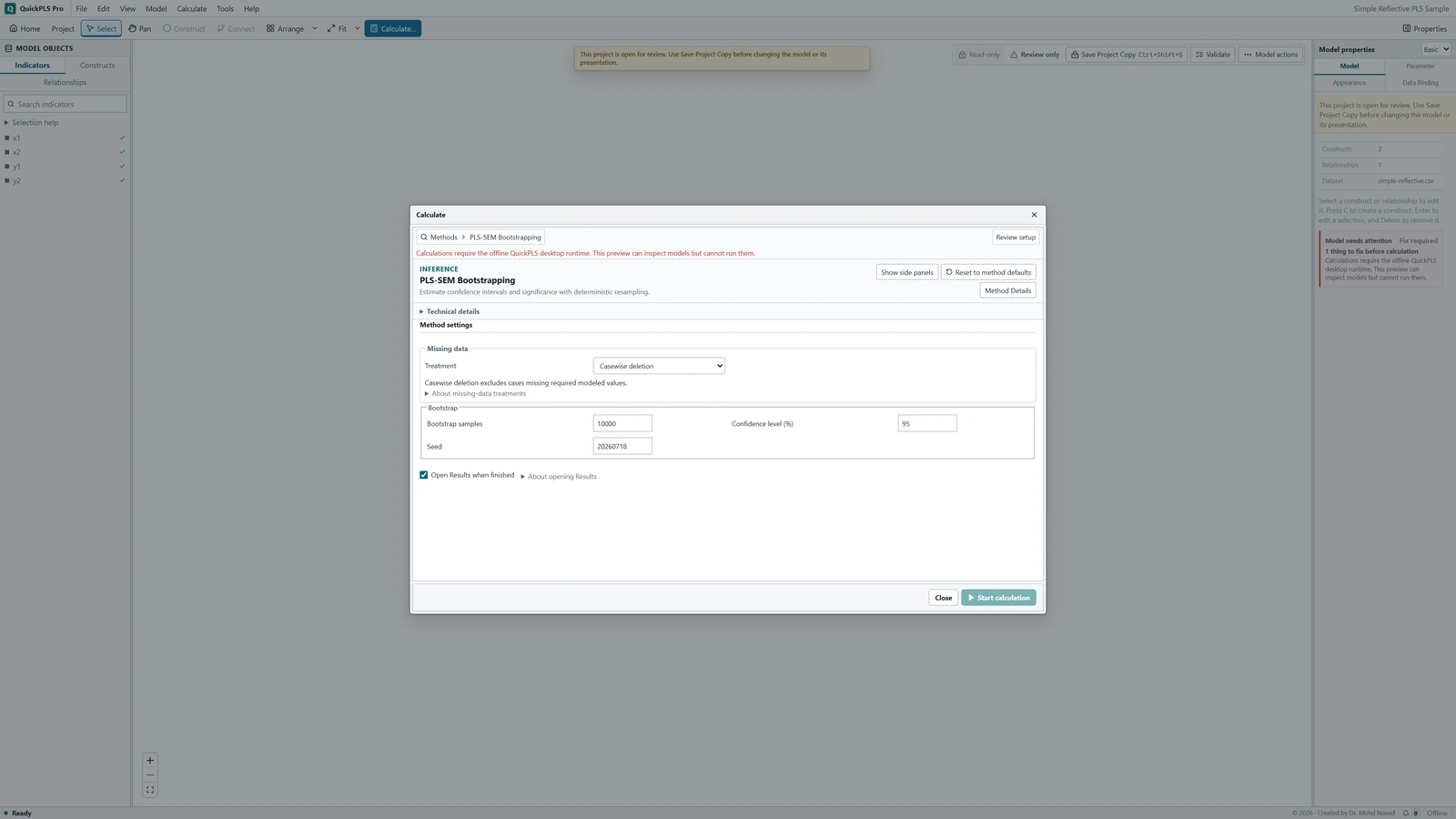
PLS-SEM Bootstrapping settings in QuickPLS. Select your own dataset and model, then use the choices described in the steps. Identify the interval you actually obtained
Read the interval name in Results. A percentile interval takes lower and upper cut-offs from the resampled estimates. Bias-corrected and accelerated (BCa) intervals also adjust for bias and for how strongly individual cases influence the estimate, using leave-one-case-out calculations. Studentized intervals scale each estimate by its uncertainty and can require another bootstrap inside every outer sample. These are explanations of interval methods, not additional selectors in this basic complete-case dialog. Report only the methods actually produced for your run.
What you should see: The interval label identifies the procedure actually returned.
How to read it: Do not rename a percentile interval as a different method.
Read the fit counts and failure reasons
Compare the requested, attempted, usable and failed sample counts. Failed fits remain in the reported counts; the procedure does not replace them with successful draws. A constant indicator has no variation in a resample; a singular equation cannot separate its predictors uniquely; nonconvergence means the fitting process did not reach its stopping rule. Check these messages before relying on an interval.
What you should see: Requested, usable and failed fits are visible.
How to read it: Investigate persistent failures before interpreting an interval.
Read paths and the indirect relationship separately
In Results, use Search result outputs to find Direct effects or Path coefficients for Quality → Satisfaction and Trust → Satisfaction. Then locate Indirect effects or Specific indirect effects and identify the complete Quality → Satisfaction → Loyalty route. Read each estimate with its own interval; two individually significant paths do not substitute for the product’s interval. Export the relevant rows and settings from this same run.
What you should see: Direct and indirect quantities have their own rows and uncertainty.
How to read it: A significant constituent path does not establish an indirect effect.
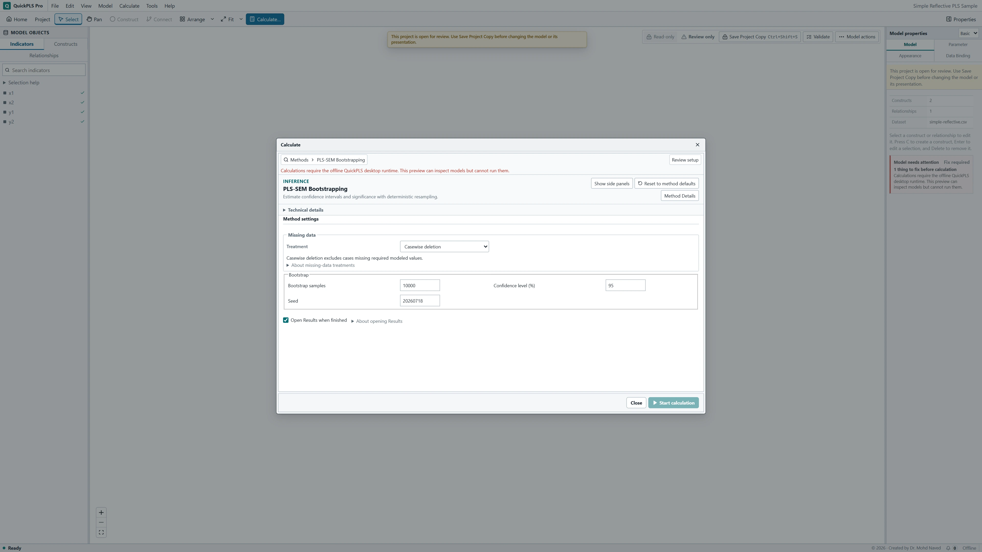
Read the estimate, its interval and the number of usable fits
The original estimate comes from your actual analysis sample. The bootstrap mean is the average estimate across usable resamples. They answer different descriptive questions, so a small difference between them is not a calculation error. Report the original estimate as the fitted relationship, alongside its uncertainty.
The standard error describes how much the estimate varies across usable resamples. It is not the spread of participants' responses and it is not the full width of a confidence interval. A confidence interval gives a range calculated by a named procedure. Over repeated comparable studies, a well-calibrated 95% procedure would cover the population value about 95% of the time. It is not a statement that 95% of participants have effects inside that range.
Read the interval method and the probability definition beside the result. A two-sided test considers departures in either direction; a one-sided test addresses a direction chosen beforehand. A test using a normal approximation and an interval based directly on bootstrap estimates need not give identical borderline decisions. Preserve the labels instead of treating every probability and interval as interchangeable.
Requested is the planned number of samples. Attempted counts the fits actually tried; usable counts the fits that supplied valid results; failed counts the rest. Read any availability message for the particular statistic as well as these overall counts.
On a small screen, swipe the table sideways to see every column.
| Output | How to read it | What to check |
|---|---|---|
| Original estimate | The coefficient from the analysed sample. | It is distinct from the mean of bootstrap estimates. |
| Standard error / interval | Variation across usable refits and the selected interval. | Check the interval method and whether the hypothesis tests one direction (one-sided) or both directions (two-sided). |
| Requested, usable and failed draws | How many samples were requested, produced usable fits or failed. | Report requested and usable draw counts separately, including failures. |
What an interval that excludes zero means
For a path coefficient, zero represents no estimated linear relationship after accounting for the other predictors in that equation. If the whole interval is positive, the result supports a positive association under the model and sampling assumptions. If the interval crosses zero, the direction is less certain.
Always ask whether the range would matter in the study. A very small association can be estimated precisely, and a potentially useful association can remain uncertain. Neither result alone establishes that changing one variable will cause another to change.
Illustrative example, not a software benchmark
A two-sided interval for a path excludes zero. Under the procedure's assumptions, that provides evidence against the corresponding zero-effect hypothesis. It does not tell you that the effect is practically important. Discuss the plausible range and what changes of that size would mean in the study.
Give readers enough information to assess the result
The related weighted PLS comparison below checks models with case weights. It is a different procedure and does not independently verify the ordinary, unweighted bootstrap taught here.
- Name the model, analysis sample and missing-data treatment. State the number of bootstrap samples, seed, confidence level and exact interval method.
- For each planned relationship, give the original estimate, standard error and interval. State the hypothesis and probability definition when reporting a test.
- Give requested, attempted, usable and failed counts, with reasons for failures or unavailable intervals. Keep the settings with the exported result so readers can tell which calculation produced it.
Use resampling to assess uncertainty
Bootstrapping reuses information from the people you observed. It cannot make an unrepresentative sample representative, turn a poorly measured concept into a reliable measure, or supply the study design needed for a causal claim.
A failed fit is useful diagnostic information. For example, a resample can leave an indicator with no variation or make two predictors too similar to estimate separate contributions. Investigate the reason, correct genuine errors and explain the remaining uncertainty. Report weak or unexpected relationships with the same attention to the question, method and interpretation as stronger findings.
Worked interpretation: a clear path and an uncertain indirect effect
Suppose a path estimate is 0.32, its bootstrap mean is 0.34 and its 95% interval is [0.14, 0.49]. The mean is 0.02 above the original estimate. The interval supports a positive association under this model, but the plausible magnitude ranges from appreciably below to above 0.32. With standardized coefficients, a path concerns change in standard-deviation units while accounting for the other predictors; it does not mean that the outcome rises by 32%. The standard error is not the interval's width.
Suppose the indirect effect is 0.08 with an interval of [-0.01, 0.18]. The range includes a small negative value, zero and positive values. A useful conclusion is: the indirect association was estimated imprecisely, and the interval included zero. That is different from showing that the mechanism is absent. Keep the planned test direction; switching to a one-sided interpretation after seeing this interval changes the question.
If 1000 samples were attempted, 960 were usable and 40 failed, report those counts together. A percentile interval can be available while BCa is unavailable because a required jackknife fit failed. A jackknife leaves out one case at a time to examine that case's influence. Studentized intervals can be unavailable because the inner standard errors are zero or unstable. Unavailable means that the calculation could not supply the requested result; it does not mean a zero effect or a probability of one.
To understand the work behind nested studentization, consider 999 outer samples with 99 inner samples each. That is 98,901 inner fits in addition to the outer fits. This is a calculation example, not an instruction to find an inner-sample field in the basic complete-case PLS bootstrap dialog. The extra fits change how uncertainty is estimated; they do not add participants.
When the interval is wide, changes sign or cannot be calculated
Start by deciding whether you have a data problem, an unstable model or an uncertain research relationship. Collinearity means that predictors overlap so strongly that their separate contributions are difficult to estimate. An almost constant item supplies very little variation. These are different problems from a valid estimate whose interval simply includes zero.
Use the table to choose a justified next step. Keep the original result before making a correction. For BCa or studentized rows, apply the advice only when that method belongs to the actual calculation you are reading; the advanced explanations do not imply that every interval is available for every model.
On a small screen, swipe the table sideways to see every column.
| Symptom | Check | Reasonable action |
|---|---|---|
| Many samples fail | Constant or almost constant indicators, collinearity and convergence messages | Correct data errors and check whether the model's parameters can be estimated from the available information. Keep failed counts visible; do not remove difficult cases merely to obtain significance. |
| The path changes sign across samples | Original coding, overlapping predictors and the width of the interval | Check whether the direction is weakly determined. Explain uncertainty instead of treating the original sign as settled. |
| BCa is unavailable but percentile exists | Availability of the leave-one-case-out jackknife calculation for the same statistic | Report the available method accurately, with the reason BCa could not be calculated. |
| Studentized bounds are missing or extreme | Inner usable counts and small or zero standard errors | Inspect numerical stability. Do not clip intervals to convenient limits or present a failed calculation as evidence of no effect. |
| A new seed changes the significance decision | How close the interval endpoint is to zero | Increase planned draws if appropriate and report the fragile conclusion. Do not search seeds for a preferred answer. |
Check stability without chasing a preferred answer
Correct a documented coding error, then rerun both the model and its bootstrap. Explain what changed and why. Removing a theoretically necessary predictor because its result is not statistically significant changes the research question. Keep both versions if an exploratory revision is useful, and describe the revised analysis as exploratory.
A useful numerical check holds the data and model fixed and uses a larger resample plan chosen in advance. More draws reduce simulation noise, meaning the variation caused by using a finite number of random draws. They do not remove the uncertainty caused by a small sample, limited measurement or biased sampling. If an interval repeatedly moves across zero with reasonable resampling plans, describe the conclusion as fragile.
Check the unit that should be resampled. Employees within a team, repeated measurements of one person and values from a time series can be related. Resampling such rows as if they were unrelated does not reproduce that dependence. Choose a sampling method that suits the design before treating the interval as evidence for a paper.
Write the methods and results in plain research language
Methods example to adapt: We fitted the prespecified reflective PLS model to the complete cases. We used case bootstrapping with 1000 attempted samples, 95% confidence intervals and seed 20261105. We recorded the interval method, sign-alignment procedure and failed fits with the exported results. Replace this template with your actual interval name, sample size and settings. Sign alignment is the calculation's procedure for keeping construct directions comparable across fits; it is not an extra switch to look for in the basic bootstrap panel.
Hypothetical Results example: The Quality to Satisfaction path was 0.32, with a 95% interval from 0.14 to 0.49. The specific indirect effect through Satisfaction was 0.08, with an interval from -0.01 to 0.18. The latter was estimated imprecisely and its interval included zero. Of 1000 attempted samples, 960 were usable and 40 failed. Add the actual failure reasons and discuss whether effects across the interval would matter in the study.
Use the table as a reporting checklist. The probability definition identifies what null hypothesis and calculation the reported probability refers to. This matters when a result includes more than one uncertainty procedure.
| Report item | What to record |
|---|---|
| Analysis sample | Cases used, exclusions and independence assumption |
| Model | Indicators, paths, estimator and weighting scheme |
| Resampling | Requested, attempted, usable and failed counts; seed |
| Uncertainty | Confidence level, exact interval method and probability definition |
| Effect rows | Original estimate, standard error, bounds and availability messages |
Can you explain your bootstrap result?
- Explain why drawing 1000 bootstrap samples reuses the original participants instead of collecting 1000 new participants.
- Find the indirect-effect interval and explain it separately from the intervals for the paths that form it.
- Show that the attempted count equals the usable count plus the failed count, and identify any unavailable statistic.
- Explain the difference between an interval that includes zero and an interval that could not be calculated.
- Save the original model, result and settings before a justified revision, so the reason for each change remains clear.