 QuickPLS
The research behind this exercise
Sherpa and colleagues studied 252 international students in South Korea using PLS-SEM. Their modified health-belief model included perceived susceptibility, severity, benefits, barriers and self-efficacy, followed by intention and adaptation. Severity was not supported in the reported model. The convenience sample was concentrated in particular demographic groups. This smaller original exercise focuses on coding, coefficient direction and the intention–behaviour distinction.
The walkthrough below is an original teaching study inspired by this methodological question. It does not reproduce the authors’ data or establish that they used QuickPLS. Read the linked paper for its complete design and findings.
The question you will answer
An international student may want to try local food but struggle with unfamiliar ingredients, access or confidence. How do perceived barriers and confidence relate to adaptation intention, and how closely does that intention relate to reported behaviour?
Larger BAR values mean more obstacles. Larger CONF values mean greater confidence in choosing unfamiliar food. INT concerns willingness, while ACT concerns reported behaviour. All three items within a block share that direction. The negative theoretical relationship from barriers is deliberate; a negative estimate is not automatically a bad result.
Treat international students as people in varied circumstances, not a single uniform group. Dietary restrictions, finances, time in the country and access to cooking facilities could matter. In a real study, choose adjustment variables because of a defensible design and avoid treating nationality as an explanation for every difference.
Step 1. Download the original practice file
The download has 260 complete fictional records: one fictional international student per row. Its continuous values sit within a 1–7 teaching response range; they are not rounded survey categories. The number of rows makes the exercise convenient to practise. It is not a sample-size recommendation for a real study.
Open the codebook before importing. Check the meanings and direction of the columns, then confirm the row count and numeric values in QuickPLS. Keep case_id only as a row identifier. It is not an indicator, predictor or control. These files have no planned missing entries, so an unexpected blank calls for an import check.
For your own study, distinguish a missing response from a genuine zero and document exclusions before analysis. Reverse a question only when its wording and scoring require it. The practice columns are already oriented as described below.
Open the import
Open a writable project and choose File → Import Data… or Ctrl+I. In Import dataset click Choose data file… and select this lesson’s CSV.
Review the preview
The dialog moves from Choose file to Review & import. Set Input represents to raw data, Header row to 1, separator to comma and Decimal convention to Dot (1.25). Confirm the teaching columns are Continuous. Keep case_id out of the analysis.
Complete the import
Check that the preview separates the columns correctly, then click Import dataset. Wait for Dataset imported and verified. Open the imported data and confirm the expected case count before building the analysis.
On a small screen, swipe the table sideways to see every column.
| Idea or role | Columns | How this exercise uses them |
|---|---|---|
| Perceived barriers | BAR1, BAR2, BAR3 | reflective construct |
| Food confidence | CONF1, CONF2, CONF3 | reflective construct |
| Adaptation intention | INT1, INT2, INT3 | reflective construct |
| Reported adaptation | ACT1, ACT2, ACT3 | reflective construct |
Step 2. Build the measurement blocks and arrows
A construct is an idea represented by several measured columns. An indicator is one of those columns. Here each three-column block is reflective: the three scores are treated as expressions of the same idea. This is a teaching assumption, not evidence that a newly written questionnaire is valid.
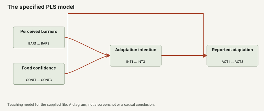
Use the exact assignments in the column table. The planned structural paths are Perceived barriers → Adaptation intention; Food confidence → Adaptation intention; Adaptation intention → Reported adaptation; Food confidence → Reported adaptation.
Create the model
With the imported data open, choose File → New Model…. Give the model a distinct name, select this lesson’s file under Dataset version, check Cases and click Create model.
Create the first block
In Indicators, click the first column of the first block. Hold Ctrl while selecting its other two columns. Check 3 selected and click Create construct.
Name it and set measurement
Choose Select and click the construct body. If needed, open View → Show Properties. Under Properties → Model enter the name from the column table and press Enter. Under Parameter → Measurement model choose Reflective.
Add the remaining blocks
Repeat that selection, naming and measurement check for every three-column block. Keep each column in its intended block. To fix an assignment, use Properties → Data Binding → Remove, then select the right column and use Assign to [construct name].
Draw and save the planned paths
Choose Connect. Drag from the body of each source construct to the body of its destination, then release. Follow the arrows listed above and return to Select. Check arrow direction and save the model. An arrow records a proposed relationship; it does not establish cause and effect.
Step 3. Run the model and find the measurement checks
PLS-SEM forms scores from the indicators and estimates the relationships in your diagram. First establish that the intended file and model can be fitted. Resampling and extensions come afterwards.
Open the calculation
Click Calculate… and enter PLS-SEM Algorithm in Find a method. Open Methods if the method list is collapsed, then select the matching row.
Check the visible choices
Use Starting weights → Standard (+1) and Missing data → Treatment → Casewise deletion. The latter keeps complete cases; the supplied file is complete. Review Readiness, leave Open Results when finished selected and click Start calculation.
Select the completed run
In Results, select the new calculation in the Result dropdown. Confirm the analysed cases and convergence. A calculation that did not settle to a stable answer needs attention before its coefficients can be interpreted.
Open the measurement tables
Open Estimates → Outer loadings, Reliability and validity → Construct reliability and validity, and Discriminant validity → HTMT+. Search result outputs can locate a table; clear the search afterwards to restore the full folder list.
Step 4. Check the fitted answers for these 260 cases
Use all 260 cases in student-food-adaptation.csv and the exact blocks and arrows in this lesson. The check uses ordinary PLS, path weighting, standardised indicators, starting weights +1, a 3,000-iteration limit and stopping criterion 0.0000001. Perceived barriers, Food confidence, Adaptation intention and Reported adaptation are reflective blocks and use Mode A.
BAR → INT is −0.359 and CONF → INT is 0.455. Higher barrier scores go with lower intention, whereas confidence goes with higher intention. INT → ACT is 0.419 after confidence is retained.
About these answers: Calculated with the QuickPLS engine and independently checked against cSEM.
On a small screen, swipe the table sideways to see every column.
| Specified path | Point estimate | Reference 95% percentile interval |
|---|---|---|
| Perceived barriers → Adaptation intention | -0.359 | -0.456 to -0.254 |
| Food confidence → Adaptation intention | 0.455 | 0.367 to 0.544 |
| Adaptation intention → Reported adaptation | 0.419 | 0.327 to 0.510 |
| Food confidence → Reported adaptation | 0.271 | 0.171 to 0.364 |
How these answers were checked
All 30 point-value comparisons and 4,000 direct-path comparisons from 1,000 common-row fits passed an absolute tolerance of 0.00000001. QuickPLS v1.03.11 calculation code and cSEM 0.7.1 fitted the same file and model directly. These checks were not new runs in the installed app. All 1,000 fits succeeded in both calculations.
The reference drew rows with R seed 261107105. Intervals use percentile endpoints with R quantile type 7. Both programs fitted the same sampled rows. This separate calculation did not use the QuickPLS bootstrap command. Entering the same seed in another program need not draw the same rows. The downloads include sampled row numbers, unrounded estimates and settings.
Step 5. Check the measurement values and explained variation
Step 5. Check the measurement values and explained variation
All blocks in this exercise are reflective. Loading relates an indicator to its construct score; Weight shows how that indicator contributes to forming the score. The presence of weights does not make these blocks formative. A high loading alone does not establish validity or distinct concepts, so also assess reliability, discriminant validity and item content.
About these answers: Point estimates calculated with QuickPLS analysis code and cSEM using the same model and data file.
On a small screen, swipe the table sideways to see every column.
| Block / indicator | Loading | Weight |
|---|---|---|
| Perceived barriers / BAR1 | 0.952 | 0.374 |
| Perceived barriers / BAR2 | 0.936 | 0.334 |
| Perceived barriers / BAR3 | 0.947 | 0.350 |
| Food confidence / CONF1 | 0.951 | 0.352 |
| Food confidence / CONF2 | 0.949 | 0.344 |
| Food confidence / CONF3 | 0.948 | 0.358 |
| Adaptation intention / INT1 | 0.946 | 0.344 |
| Adaptation intention / INT2 | 0.952 | 0.352 |
| Adaptation intention / INT3 | 0.951 | 0.357 |
| Reported adaptation / ACT1 | 0.948 | 0.341 |
| Reported adaptation / ACT2 | 0.951 | 0.350 |
| Reported adaptation / ACT3 | 0.951 | 0.361 |
Explained variation in each outcome
R² describes this fitted sample. It is not a test of prediction on new observations.
| Outcome | R² |
|---|---|
| Adaptation intention | 0.364 |
| Reported adaptation | 0.359 |
Read each indirect route separately
Each row follows one specific route. Multiply its component coefficients within each repeated fit before taking the interval; multiplying the endpoints of component intervals is incorrect. These are statistical associations in synthetic data, not evidence of causal mediation.
About these answers: Indirect effects recalculated for each shared resampled dataset. These reference intervals are not QuickPLS bootstrap output.
On a small screen, swipe the table sideways to see every column.
| Specific route | Point product | Reference 95% percentile interval |
|---|---|---|
| Perceived barriers → Adaptation intention → Reported adaptation | -0.151 | -0.206 to -0.100 |
| Food confidence → Adaptation intention → Reported adaptation | 0.191 | 0.136 to 0.259 |
Step 6. Check the questions before explaining the arrows
Read the BAR item definitions before interpreting its loadings or path. An item about easy access would run in the opposite direction to an item about difficulty finding suitable food. The supplied BAR scores already mean greater barriers; do not reverse them because you expected a positive coefficient.
Read a loading with the meaning and direction of its item. Reliability concerns how consistently a block works together. Average variance extracted, or AVE, summarises how much indicator variation the reflective block represents. HTMT+ compares pairs of reflective constructs and helps you investigate whether supposedly different ideas are too alike.
Open Collinearity and effects → Inner VIF values for predictors entering the same outcome. Strong overlap makes their separate contributions harder to distinguish. A threshold is a prompt to investigate, not a replacement for reading the item definitions. Record concerns before inspecting which hypothesis looks attractive.
Step 7. Add intervals for the planned relationships
Return to Calculate… and choose PLS-SEM Bootstrapping. For this repeatable practice run set Bootstrap samples to 1000, Confidence level (%) to 95 and Seed to 261107105. These are teaching choices, not a claim that the paper used them or that 1000 draws is always enough for final research.
Start the calculation and inspect requested, attempted, usable and failed draws. A bootstrap repeatedly draws complete rows with replacement and refits the model. Read the interval name and test definition supplied with the result; the basic complete-case panel does not provide the separate PLSc interval selectors.
Open Effects → Direct effects for the drawn arrows. For a pathway through an intermediate construct, find its named specific indirect effect and use that row’s interval. Open Estimates → R-squared for explained variation and Collinearity and effects → f-square effect sizes for each predictor’s contribution. Keep the original estimate, interval and output label together.
Step 8. Check direction before checking significance
Make a small coding note: high BAR means more obstacles; high INT means greater willingness. Under the stated hypothesis, a negative BAR → INT coefficient is consistent with the expected direction. A positive number would need explanation rather than automatic relabelling.
For a genuinely reverse-worded item on a 1–7 scale, a reversal would be 8 minus the observed response. That transformation is justified only by the instrument’s scoring rule. Applying it to every barrier item simply to make the arrow positive would change what the construct means.
Step 9. Turn a coefficient into a careful sentence
Read Effects → Direct effects and locate BAR → INT using the construct names. Check which other predictor enters Intention: Food confidence. The coefficient describes barriers while accounting for that included confidence factor. It is not the same as the unadjusted relationship between the two scores.
Hypothetical example
Illustrative reading example
Suppose the standardized Barriers → Intention coefficient is -0.28, with a 95% interval from -0.43 to -0.10. Greater barriers are associated with lower intention under this model. Suppose Intention → Reported adaptation is 0.35, with an interval from 0.14 to 0.54. That supports an association, not a claim that 35% of students changed their diet. These are invented interpretation examples.
Step 10. Do not let intention stand in for behaviour
A participant can want to adapt while continuing familiar habits. Read the Intention and Reported adaptation measurement blocks separately, and inspect R-squared for each outcome. A model may explain willingness well but leave much of actual behaviour unexplained.
The synthetic ACT block represents a self-report, not meal records. A stronger follow-up design might collect a clearly defined period of behaviour after the intention measure. If the research question concerns nutrition or health, additional measures and expertise are needed; adaptation itself is not a health outcome.
What to check when the result is unexpected
If the barrier path is positive, check scale direction, wrong item assignments, predictor overlap and the composition of the sample before telling a story. A conditional sign can differ from a simple correlation when predictors overlap. Read Inner VIF values and the substantive model together.
If a single item points the opposite way, inspect its source coding. Correct an actual error in a separately saved file and refit the model. Do not delete honest students with unusual preferences to make the sign match a hypothesis.
If the intention–behaviour path is uncertain, consider whether the measures refer to the same activity and time period. A wide interval is different from evidence that willingness never matters.
Save the original model and the reason for each genuine correction. Keep unsupported relationships in the results you report. A more convincing study explains a weak or uncertain finding and plans better evidence; it does not erase cases, items or paths until every test is favourable.
Step 11. Write a clear Methods and Results account
Methods outline: We defined higher barrier scores as more obstacles and checked item direction before fitting the reflective model. Barriers and Food confidence predicted Adaptation intention; Intention and Confidence predicted Reported adaptation. We used [settings] and [uncertainty method].
Results outline: The barrier coefficient was [value and interval], conditional on Confidence. Intention was related to Reported adaptation by [value and interval]. Our outcome records [exact behaviour definition and period], so the conclusion concerns [scope].
Include the analysed case count, exact file or data version, model diagram, measurement decisions, calculation settings and the uncertainty procedure. Attach the relevant full tables rather than only the strongest row. Explain which decisions were planned and which followed inspection.
For this exercise, call the records simulated teaching data. In an actual paper, replace every bracketed placeholder with the result from the named saved run. Remove any illustrative numbers from this lesson before drafting your findings. Cite the original study for the research context and the relevant methodological references for the analysis.
Step 12. Put this result into a report
We fitted the specified ordinary PLS model to 260 original synthetic teaching cases. The measurement roles and complete structural model were fixed before interpreting the results. Point estimates were checked against an independent cSEM calculation.
Report each path estimate with its matching interval. If you use the reference intervals here, explain that both programs fitted the same resampled datasets in a separate checking procedure. Do not describe them as results from a QuickPLS command you have not run. For a real study, add the sampling design, measurement evidence and reasons for the model choices.
Check your conclusion before you finish
- Explain why a negative barrier coefficient can support the hypothesis.
- Keep reverse coding tied to item wording.
- Distinguish intention, self-reported behaviour and objective behaviour.
- Report who the sample represents without generalising to all international students.