 QuickPLS
A group difference needs comparable measurement
Dong, Veloutsou and Morgan-Thomas studied negative brand responses and brand happiness using a consumer survey, covariance-based structural modelling and a comparison of consumer clusters. Their quantitative sample contained 513 respondents. The paper includes measurement-invariance stages before structural comparisons.
In QuickPLS you will fit the measurement model, review its invariance across the two groups and compare one structural path on their common factor scale. The original teaching groups let you practise that sequence without reproducing the paper’s consumer clusters. Because the source’s reported degrees of freedom leave some single-path comparisons unclear, this exercise declares the equality explicitly and checks the actual restrictions in its own output.
Your study: does anger relate to complaint intention differently?
Imagine 400 fictional consumers rating brand disappointment, negative feeling and constructive complaint intention. Each factor has three reflective continuous 1–7 teaching indicators. GROUP contains independent A and B labels assigned for practice. They are not discovered consumer segments, and no genuine group difference is promised.
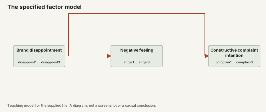
The planned structural model is Disappointment → Anger, Anger → Complaint intention and Disappointment → Complaint intention. The comparison asks whether the unstandardized Anger → Complaint intention coefficient differs between A and B on a common factor scale.
First fit a measurement-only confirmatory factor analysis, or CFA, with the three factors allowed to covary. Then examine measurement comparability across groups. Only after reviewing that evidence should you compare the structural path. Different diagram labels do not guarantee different psychological constructs, and identical labels do not guarantee comparable measurement.
On a small screen, swipe the table sideways to see every column.
| Role | Columns | Use |
|---|---|---|
| Disappointment | disappoint1, disappoint2, disappoint3 | Reflective factor |
| Anger | anger1, anger2, anger3 | Reflective factor |
| Complaint intention | complain1, complain2, complain3 | Reflective factor |
| Group | GROUP: A or B | Independent teaching groups; not an indicator |
| Identifier | case_id | Case label only |
Step 1. Import the scores and preserve the actual group values
Use a writable project and choose File → Import Data… → Choose data file…. In Review & import select raw data, Header row 1, comma separation and Decimal convention Dot (1.25). Keep the nine measurement columns Continuous. Preserve GROUP as its actual A/B categories, then choose Import dataset and verify 400 cases.
The scores are complete and already point in their stated direction. Keep GROUP and case_id outside the indicator assignments. Check group counts in the imported data and again in every analysis. Do not infer counts merely from the total sample size.
For a real study, groups need a defensible meaning and independent observations. If groups were discovered from the same outcomes later compared, interpretation requires particular care about selection. Here the independent teaching labels let you learn the mechanics without claiming substantive consumer segments.
Step 2. Save a common three-factor measurement model
Maximum likelihood is the fitting method used here for the continuous teaching data. It is not an ordinal or complex-survey correction. Keep the marker choices and factor directions unchanged across the later grouped analyses. No residual covariance is added merely to improve a fit index.
Create and identify the common factors
Choose File → New Model… for the imported Dataset version. Create each block from its three matching columns using Indicators → Create construct. Name the blocks in Properties → Model. Set Inspector mode to Expert, choose Parameter → Measurement model → Reflective, then Scientific representation → Representation → Common factor. Set Marker indicator to disappoint1, anger1 and complain1 for their respective factors. Each marker loading is fixed at 1 to set scale.
Add the three CFA covariances
Leave out the directed research paths. Use Connect to drag between each factor pair, return to Select and click the relationship. Under Properties → Parameter set Relationship type to Covariance. Under Relationship use select Use → Model covariance and click Apply relationship use. Repeat for Disappointment ↔ Anger, Disappointment ↔ Complaint intention and Anger ↔ Complaint intention. Save the CFA model.
Fit and inspect the CFA
Choose Calculate… → CB-SEM / CFA. Set Estimation workflow to Existing CFA / recursive SEM and Inference to Maximum-likelihood point estimates. Check Model topology says Confirmatory factor analysis. Review the dataset, complete-case preparation and Readiness, then choose Start calculation. Inspect convergence, loadings, factor relationships, residual variances, standard errors and fit before saving the usable result.
Step 3. Run the grouped measurement hierarchy
Before starting, confirm that the saved setup uses this lesson’s three factors, GROUP values A and B, and the selected Configural → Metric → Scalar hierarchy. In the preview, check group counts and exclusions against the imported file. The later structural comparison must use measurement evidence from these same groups and indicators.
Prepare the grouped CFA
Choose Calculate… → CB-SEM Measurement Invariance → Prepare a new invariance setup. Select the Saved single-group CFA model, enter a New setup name and choose GROUP as Grouping variable.
Declare groups and stages
Enter Reference value A and Reference label Group A, then Compared value B and Compared label Group B, matching the stored category type. Select Configural → Metric → Scalar under Invariance hierarchy. Read and select the checkbox adding missing observed intercepts while preserving existing parameter specifications. Leave the optional joint latent-mean test off for this path-comparison exercise.
Preview, save and calculate
Choose Preview setup and check group counts and exclusions. Choose Save new setup, Use saved setup and Check saved setup. Then choose Start calculation and Open Results.
Step 4. Read the first usable stage before the stronger restrictions
Search Results for Group populations, Measurement invariance fits, Adjacent comparisons and Stage parameter estimates. Configural uses the same indicator-to-factor pattern. Metric adds equal corresponding free loadings. Scalar also adds equal intercepts, which concerns the response baselines needed for latent-mean interpretation.
For the planned structural-path comparison, review whether metric equality provides a defensible common scale. Scalar evidence answers an additional measurement question; this lesson does not compare factor means. A poor configural model should be investigated before stronger equalities are treated as meaningful.
If a named item works differently for a substantive reason, a partial-invariance follow-up may be justified. Preserve the full result, name the released equality and explain the reason. Do not repeatedly free parameters until a convenient cutoff appears. A partial model must retain enough common information to support the intended comparison.
Hypothetical example
Illustrative reading example
Suppose configural, metric and scalar chi-square values are 180, 188 and 199, on 48, 54 and 60 degrees of freedom. The adjacent changes are 8 on 6 degrees of freedom and then 11 on 6. These invented values illustrate checking what each stage adds. They are neither the paper’s statistics nor fitted answers for the teaching file.
Step 5. Save the structural model with the same measurement
Do not change an indicator between the invariance analysis and the structural comparison while continuing to cite the old measurement result. The evidence must match the actual factor pattern, cases and groups. If measurement changes, repeat the relevant measurement review.
Choose Anger → Complaint intention as the single planned target. Keep the comparison on the unstandardized factor scale established by the markers. Standardized coefficients can differ partly because groups have different variances, so they should not silently replace the declared unstandardized contrast.
Create the structural specification separately
Choose File → New Model… for the same dataset. Recreate the three blocks with the same Reflective measurement, Expert Common factor representation and marker indicators. Use Connect to draw Disappointment → Anger, Anger → Complaint intention and Disappointment → Complaint intention. Return to Select and save. Disappointment is the only exogenous factor, so do not transfer the CFA’s three factor covariances.
Fit the structural model
Choose Calculate… → CB-SEM / CFA. Set Estimation workflow to Continuous-linear structural ML, Moment structure to Covariances and Inference to Maximum-likelihood point estimates. For practice use Maximum iterations per stage 1000 and Convergence tolerance 0.0000001. Under Numerical solver choose Solver → Improved convergence. Review Readiness, start calculation and inspect convergence, parameters, residual variances and fit.
Step 6. Declare and run the single-path comparison
Create the multigroup setup
Choose Calculate… → CB-SEM Multigroup Analysis → Prepare a new multigroup setup. Select the Saved structural model, enter a New setup name and choose the Reviewed full invariance result.
Choose the path and retained measurement
Select Anger → Complaint intention under Structural path to compare. Under Metric constraints to retain choose the full metric constraints, or a compatible justified partial-metric follow-up linked to that full result. Under Declared path equalities put A and B in Equality block 1.
What you should see: Anger → Complaint intention is the sole declared path comparison, with A and B sharing the stated metric constraints.
Complete the review after the choices are final
Check the inherited group order and intended A-minus-B contrast. Enter the Reason for accepting metric invariance and complete the review confirmation. Read and select the checkbox copying grouping and missing indicator intercepts while preserving existing parameters. Changing the path, evidence or blocks requires the review confirmation again.
Set the uncertainty and calculate
Under Stratified full-ML bootstrap request 1000 Bootstrap draws, Seed 202611083 and a 95% Pointwise confidence level; record Workers. Choose Preview setup, Save new setup, Use saved setup and Check saved setup and review. Start calculation, then Open Results and inspect refit diagnostics before the contrast.
Check the factor models for these 400 cases
Use continuous maximum likelihood with the first indicator loading fixed to 1 for each factor. The CFA allows every factor pair to covary. The structural model retains only the paths and exogenous-factor covariances listed in this lesson. No indicator residual covariance is added.
Review the configural, metric and scalar measurement results before interpreting a group difference. The grouped structural result below retains full metric loading equalities, with the first loading fixed to 1 in both groups. Scalar constraints are assessed separately and are not silently added to this path comparison.
About these answers: Comparison answers calculated in lavaan 0.7.3, with independent checks of covariances and standardised estimates.
On a small screen, swipe the table sideways to see every column.
| Saved model | Chi-square / df | CFI | RMSEA | SRMR |
|---|---|---|---|---|
| cfa | 15.547 / 24 | 1.000 | 0.000 | 0.012 |
| structural | 15.547 / 24 | 1.000 | 0.000 | 0.012 |
| configural | 42.407 / 48 | 1.000 | 0.000 | 0.019 |
| metric | 50.585 / 54 | 1.000 | 0.000 | 0.026 |
| scalar | 63.625 / 60 | 0.999 | 0.017 | 0.028 |
| group structural | 50.585 / 54 | 1.000 | 0.000 | 0.026 |
What these checks establish
All reference models converged and passed lavaan’s check for allowable parameter estimates. A separate calculation reconstructed the covariances predicted by each model, the observed covariances, standardised loadings and paths, and the maximum-likelihood discrepancy used to assess fit. It did not independently refit the model or check the standard errors used for the Wald intervals.
The reference uses continuous maximum likelihood and fixes each first loading at 1 to set the factor’s scale. Ungrouped runs fit the covariances; grouped runs also include intercepts. The supplied individual-path intervals are normal-theory Wald intervals, not bootstrap intervals.
A CFI rounded to 1 or RMSEA of 0 is not a certificate that the theory is true. Read the residuals, measurement meaning and design alongside overall fit. The download retains all parameters, warnings and covariance records.
Read the structural estimates on the right scale
The raw coefficient uses the marker-defined factor unit. The standardised coefficient uses standard-deviation units. The displayed interval belongs to the raw estimate; do not attach it to the standardised value.
About these answers: External ML point estimates. The intervals below are normal-theory Wald intervals, not the case-bootstrap intervals requested later in the app lesson.
On a small screen, swipe the table sideways to see every column.
| Path | Raw estimate | Standardised estimate | Raw 95% Wald interval |
|---|---|---|---|
| Group A / Brand disappointment → Negative feeling | 0.525 | 0.523 | 0.393 to 0.656 |
| Group A / Negative feeling → Constructive complaint intention | 0.487 | 0.455 | 0.313 to 0.661 |
| Group A / Brand disappointment → Constructive complaint intention | -0.027 | -0.026 | -0.199 to 0.144 |
| Group B / Brand disappointment → Negative feeling | 0.424 | 0.429 | 0.290 to 0.558 |
| Group B / Negative feeling → Constructive complaint intention | 0.386 | 0.414 | 0.244 to 0.527 |
| Group B / Brand disappointment → Constructive complaint intention | 0.029 | 0.031 | -0.110 to 0.167 |
Check the CFA measurement values
Check the CFA measurement values
The first raw loading is fixed at 1 to set each factor’s scale. Its standardised value can differ from 1. The other loadings are estimated.
About these answers: Measurement-only CFA from lavaan; not the structural model or a PLS loading table.
On a small screen, swipe the table sideways to see every column.
| Factor / indicator | Raw loading | Standardised loading |
|---|---|---|
| Brand disappointment / disappoint1 | 1.000 | 0.921 |
| Brand disappointment / disappoint2 | 1.002 | 0.926 |
| Brand disappointment / disappoint3 | 1.013 | 0.932 |
| Negative feeling / anger1 | 1.000 | 0.926 |
| Negative feeling / anger2 | 0.995 | 0.914 |
| Negative feeling / anger3 | 0.993 | 0.916 |
| Constructive complaint intention / complain1 | 1.000 | 0.922 |
| Constructive complaint intention / complain2 | 0.995 | 0.916 |
| Constructive complaint intention / complain3 | 1.001 | 0.918 |
Test the difference itself, not two significance labels
For anger → complain, the raw estimate is 0.487 in A and 0.386 in B. The A-minus-B contrast is 0.101, with a 95% reference percentile interval of -0.093 to 0.291. The interval includes zero: this file does not provide clear evidence of a group difference for that path.
Both groups use the same first-indicator marker and full metric loading equalities. These are raw factor-unit coefficients, not standardised group coefficients. The bootstrap resamples cases within each group and refits the full constrained model.
About these answers: External lavaan reference with 1,000 complete stratified ML refits. Contrast arithmetic and interval endpoints independently checked.
| Quantity | Estimate / interval |
|---|---|
| A minus B | 0.101 |
| 95% reference percentile interval | -0.093 to 0.291 |
| Joint-model Wald standard error | 0.113 |
| Joint-model Wald two-sided p-value | 0.371 |
| Requested / usable stratified fits | 1000 / 1000 |
What belongs to this group contrast
Reference seed 202611083; 1,000 stratified resamples; percentile endpoints. Metric loading equalities are retained, while group intercepts are not constrained equal. The jointly fitted model supplies the Wald covariance, so its standard error is not formed by assuming two independent path estimates.
Arithmetic of all retained paired A-minus-B contrasts and percentile endpoints independently checked. The ML fits and Wald covariance are external lavaan references, not independently optimized or run in QuickPLS.
The saved model and resample ledger retain all warnings and failures. This reference does not turn measurement invariance into proof of causality or population equality.
Step 7. Use the contrast’s own interval
Open Group path estimates, then Declared path contrasts. Read the subtraction order printed in the result. A positive A-minus-B estimate means the path is larger in A on the stated common scale. Its interval is the uncertainty for that difference.
Read Declared path-equality test as the test of the restriction actually imposed. One freely estimated path made equal across two groups ordinarily adds one independent restriction when all other specifications are held fixed. If the reported degrees-of-freedom change differs, inspect what else changed before calling it a single-path test.
The within-group bootstrap resamples cases separately inside their original groups and refits the full model. Report usable and failed refits. A large overall sample does not automatically compensate for a very small or unstable group, and a failed constrained fit must not be silently replaced by another model.
Hypothetical example
Illustrative reading example
Suppose the unstandardized Anger path is 0.35 in A and 0.22 in B. A minus B is 0.13. If its 95% interval is [-0.06, 0.31], the direction of the group difference remains uncertain. A path being significant in A and not in B would not override that contrast. These are hypothetical values, not generated group differences.
Resolve measurement and comparison problems first
On a small screen, swipe the table sideways to see every column.
| Observation | Check | Action |
|---|---|---|
| One configural group fit is poor | Coding, factor pattern, group size and improper estimates | Investigate before imposing metric or scalar equality. |
| Metric equality looks questionable | Named loadings and their content across groups | Explain a justified partial follow-up or limit the structural comparison. |
| The structural setup rejects the invariance result | Matching indicators, markers, groups and linked full result | Use compatible evidence or repeat the necessary measurement analysis. |
| The contrast sign seems reversed | A-minus-B order and factor orientation | Match the printed order in the table and prose. |
| A supposed single-path test has unexpected degrees of freedom | All restrictions and specifications that changed | Report the actual joint change; do not label it one path without checking. |
| The difference interval crosses zero | Its range and practical meaning | Report uncertainty, not proof of group equivalence. |
Keep a measurement revision separate from a search for group effects
If content justifies a partial metric model, compare its planned path contrast with the full-metric result and describe the retained common scale. Show both analyses. Releasing whichever loading makes the path difference significant is exploratory searching, not confirmation of the original group hypothesis.
The teaching groups were assigned independently and were not designed to differ. A null or uncertain comparison is therefore a useful exercise outcome. Do not reassign cases to obtain a contrast. In real research, explain why the groups exist and what alternative explanations could account for a difference.
Report the measurement basis and the path contrast together
Methods outline: We fitted a three-factor continuous-ML CFA with [markers] in independent groups A and B. We examined configural, metric and scalar stages and retained [measurement equalities and reason] for the structural comparison. We compared Anger → Complaint intention using the A-minus-B contrast and a stratified full-ML bootstrap with [settings and usable counts].
Results outline: The measurement review indicated [stage-specific findings]. The group path estimates were [A] and [B], giving a contrast of [difference] with a 95% pointwise interval of [bounds]. The declared equality test imposed [actual restrictions and degrees of freedom]. [Explain uncertainty or any incompatibility.] These arbitrary teaching groups are not substantive consumer segments.
| Report item | Include |
|---|---|
| Groups | Actual values, definitions, counts and independence. |
| Measurement | Factor pattern, markers and full or partial invariance evidence. |
| Structural target | One named path on a common unstandardized scale. |
| Contrast | Subtraction order, estimate and matching interval. |
| Restriction test | Actual equality restrictions, statistic and degrees of freedom. |
| Refits | Requested, usable and failed within-group bootstrap fits. |
Explain the model comparison
We fitted the stated CFA and structural model to 400 synthetic teaching cases using continuous maximum likelihood and first-indicator markers. We kept the CFA measurement covariances separate from the structural specification.
Report fit and measurement evidence before the paths. Label the individual-path intervals as normal-theory Wald intervals. Label the A-minus-B interval as a percentile interval from the separate 1,000-refit stratified reference; the joint-model Wald standard error and p-value are different results. The lesson’s app bootstrap remains a separate procedure with its own usable counts, failures and intervals.
Check the group claim against the actual analysis
- Explain what becomes equal at the metric and scalar stages.
- Find the measurement result linked to the structural comparison.
- Recalculate the actual A-minus-B contrast of 0.101 from the reference group estimates, allowing for display rounding, and read its own percentile interval. Then use the separate 0.13 example as an optional arithmetic check.
- Explain why separate significance markers cannot establish a group difference.
- Identify exactly how many independent restrictions the declared test added.
- Keep the full and any justified partial measurement results available.