 QuickPLS
What the method does
Multigroup analysis fits related models to different groups and tests selected parameter differences. A different estimate in two groups is not enough to establish a statistically supported difference. Measurement comparability, compatible specifications and a direct test of the contrast are needed.
Path contrast: Δb = bgroup 1 − bgroup 2.
The sign depends on the stated group order. Uncertainty for Δb answers whether the estimates differ; separate within-group p-values answer different questions. Equality constraints can test the selected contrast in an identified multigroup model.
Data and analysis in QuickPLS
Use case-level indicators plus a group column. Check measurement invariance at the level required for the proposed comparison and adequate usable cases in every group.
QuickPLS lets you select the groups and the parameters to compare. Read both group estimates, their order and the direct contrast result together.
Follow a worked example
The following example shows the data, settings and decisions for one analysis. Use the linked practice files to follow it. For your own study, keep the procedure and choose the variables, model and settings that fit your research question.
Download research-workshop.csv to begin. It contains 360 rows and 31 columns. The example below identifies the variables to use, their roles and any rows to exclude; not every column is an analysis variable.
Is the Satisfaction-to-Loyalty relationship different between groups?
Imagine that Satisfaction appears more strongly related to Loyalty in one group. To assess that claim, compare the two path coefficients directly. A path being statistically significant in one group and not significant in the other does not establish a difference between them.
First check that both groups use a comparable measurement scale. Metric invariance means that the corresponding factor loadings can be treated as equal. Review that evidence before comparing structural paths, the relationships drawn between factors.
The analysis estimates uncertainty by repeatedly sampling cases with replacement within their original groups and fitting the full maximum-likelihood model again. A case can appear more than once in a resample. This is a stratified bootstrap. The interval for the path difference shows how precisely the data distinguish the groups on the stated scale.
Bring a structural model and its measurement review
Save the common structural model and complete the full measurement-invariance analysis for the same factors, indicators and independent groups. Decide which path to compare, which groups should share a path in the restricted model, and the order in which their estimates will be subtracted.
Use full metric constraints, or a compatible partial-metric follow-up tied to that full invariance result. Keep marker indicators and factor direction consistent. Selecting a saved result records where the evidence comes from; you still need to explain why you accept its measurement assumptions.
Before starting, identify three saved items by name: the common structural model, the full measurement-invariance result and any partial-metric follow-up you intend to use. The comparison must use the same factors, indicators and groups as that evidence.
Connect the path comparison to the reviewed measurement model
Prepare the structural setup
Click Calculate… → CB-SEM Multigroup Analysis → Prepare a new multigroup setup. Choose the Saved structural model, enter a New setup name and choose the Reviewed full invariance result.
Declare the path and comparison assumptions
Choose the Structural path to compare and Metric constraints to retain. Under Declared path equalities, place the groups to be compared in the same Equality block. The grouping and group order come from the reviewed setup. Once those choices are settled, record the Reason for accepting metric invariance and complete the required review decisions. Changing the path, evidence or equality blocks clears the review confirmation, so confirm it again after any change.
Set uncertainty, save and calculate
Under Stratified full-ML bootstrap set Bootstrap draws, Seed, Workers and the Pointwise confidence level where shown. Use Preview setup, Save new setup and Use saved setup. Check the saved choices with Check saved setup and review, then click Start calculation. After Open Results, read the group paths, direct contrasts and refit diagnostics together.
Read the contrast, not the separate significance markers
After Open Results, search for Group path estimates to see the association in each group. Then open Declared path contrasts. Its label tells you which coefficient is subtracted from which. Read the contrast estimate and its own interval before making a group-difference claim.
For the declared single-path analysis, Declared path-equality test assesses the planned equality restriction. The joint-path option has a separate Joint path-equality test. These likelihood-ratio tests and the pointwise bootstrap intervals answer related but distinct questions.
Check Group populations, the measurement review and the bootstrap counts before relying on uncertainty. A model that fails or gives impossible estimates in one group needs investigation; replacing it silently with a different model would change the comparison.
On a small screen, swipe the table sideways to see every column.
| Output | How to read it | What to check |
|---|---|---|
| Group-specific path | The selected path estimate in each specified group. | Check that the parameters can be estimated and that their scales allow a meaningful comparison across groups. |
| Path difference / interval | The estimated difference between the selected groups. | Read the order of subtraction and interval procedure. |
| Invariance and refit diagnostics | Measurement checks and the number of successful full-model refits supporting the interval. | Do not replace a failed constrained fit with an unexplained alternative. |

The difference needs its own uncertainty
Even when both path estimates are known, their separate significance levels do not tell you whether they differ from each other. Read the direct difference and its interval. The example below isolates the arithmetic so you can identify the quantity that answers the group question.
Illustrative example, not a software benchmark
If the group estimates are 0.30 and 0.20, the difference is 0.10. Its uncertainty depends on both estimates and the comparison procedure. The separate probability for each path cannot tell you the uncertainty of that difference. These numbers illustrate the calculation; they are not a software benchmark.
Practice: compare Satisfaction → Loyalty in groups 0 and 1
Use research-workshop.csv with the four reflective blocks and the paths Quality → Satisfaction, Trust → Satisfaction and Satisfaction → Loyalty. The teaching groups are independent synthetic groups 0 and 1. Run and review the measurement-invariance analysis for these same blocks and groups first.
Use the same four Common factor blocks and first-indicator markers as the invariance exercise. For the structural model retain only Quality → Satisfaction, Trust → Satisfaction and Satisfaction → Loyalty, plus the covariance between exogenous Quality and Trust. Keep the same specification in both groups. Choose Satisfaction → Loyalty as the planned target. Define the contrast as group 0 minus group 1 so that a positive difference means a larger coefficient in group 0.
This lesson asks about the direct difference. Two separate tests of whether each path equals zero would answer different questions. For a study with more paths or more groups, plan the joint restrictions and contrasts first; the supported range is 2 to 32 independent groups.
Prepare, review and run the declared comparison
Check the common structural model
Fit the continuous reflective model and inspect its estimates. Match the indicators, factors, marker scales and grouping data to the saved invariance analysis. If you change an indicator, review the measurement evidence again instead of attaching the old result to a different model.
What you should see: The groups share the intended structural specification.
How to read it: Resolve incompatible indicators or paths before testing differences.
Open a new multigroup setup
Choose Calculate… → CB-SEM Multigroup Analysis → Prepare a new multigroup setup. Select the Saved structural model and enter a New setup name that identifies the Satisfaction-to-Loyalty comparison.
What you should see: The multigroup setup identifies the correct dataset and group field.
How to read it: Check group labels and usable counts.
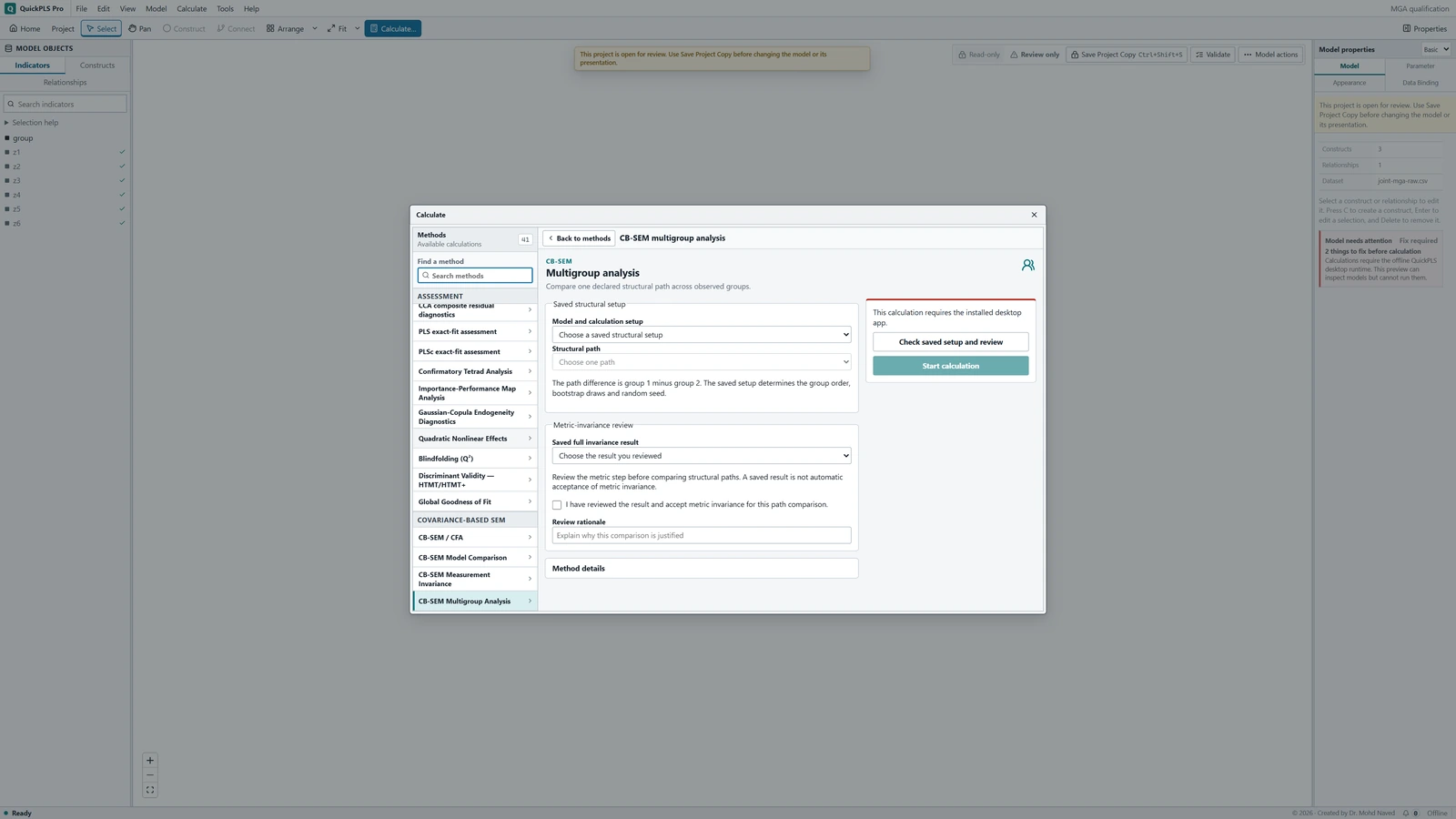
CB-SEM Multigroup Analysis settings in QuickPLS. Select your own dataset and model, then use the choices described in the steps. Choose the measurement evidence
Select the Reviewed full invariance result. Under Metric constraints to retain choose Full metric constraints, or the saved compatible partial-metric follow-up linked to that exact full result. Read the measurement evidence and decide why it supports this comparison. Complete the review confirmation after the path and equality blocks are final.
What you should see: The measurement evidence matches the comparison being requested.
How to read it: Do not infer comparable measurement from path similarity.
Declare the comparison between groups
Choose Satisfaction → Loyalty under Structural path to compare. In Declared path equalities, assign both groups to Equality block 1. Check the inherited order: the first group minus the other gives group 0 minus group 1. For several paths, Compare several paths in one joint test opens separate choices and equality blocks. Now complete the metric-review checkbox and Reason for accepting metric invariance. For this exercise, read and select the checkbox permitting the setup to copy grouping and missing indicator intercepts while preserving existing parameters. If you change the path, evidence or blocks afterwards, confirm the review again.
What you should see: The requested path contrast and group order are explicit.
How to read it: A direct contrast is needed to establish a between-group difference.
Choose the bootstrap settings
Under Stratified full-ML bootstrap enter 1000 Bootstrap draws for the teaching run and record Seed and Workers. Choose the Pointwise confidence level before looking at the contrast; the declared-group workflow offers 90%, 95% and 99%. The reporting example below uses 95%. More draws improve a resampling summary but do not make the sample larger.
What you should see: The bootstrap settings match the group comparison.
How to read it: Record the draw count, confidence level and seed.
Preview, save, check and run
Click Preview setup and review the group counts and measurement compatibility. Click Save new setup, then Use saved setup. Check the selected model and review with Check saved setup and review, then Start calculation. After Open Results, inspect the fits and failed refits before interpreting the contrasts.
What you should see: The saved result includes both group estimates and the contrast.
How to read it: Interpret its interval rather than comparing separate significance labels.
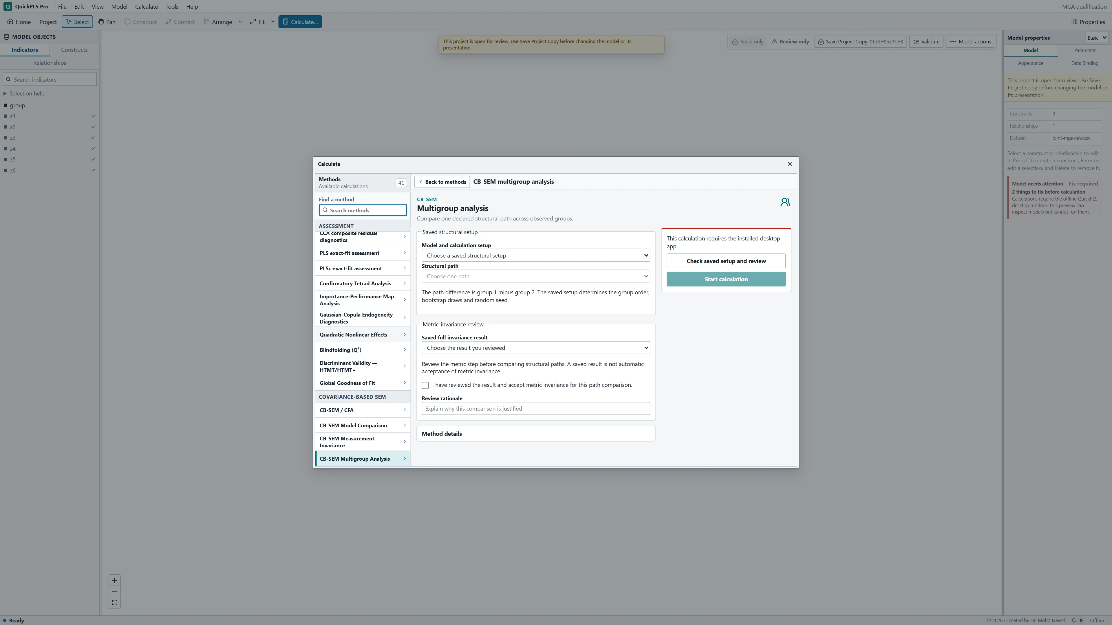
Turn the contrast into a clear research statement
Suppose the unstandardized Satisfaction → Loyalty coefficients are hypothetically 0.30 in group 0 and 0.20 in group 1. Unstandardized means the coefficients use the model's factor units. On a comparable scale, group 0 minus group 1 is 0.10. If its 95% interval runs from -0.04 to 0.24, the evidence leaves both negative and positive differences plausible at that interval level.
The interval includes zero, so it does not establish a direction for the group difference. That is not proof that the groups are equivalent: practically relevant differences may still lie inside the interval. Report the range and its meaning rather than describing an uncertain result as no relationship.
Reversing the order changes 0.10 to -0.10 and reverses the interval accordingly. Check the contrast label before writing the conclusion. Keep the scale consistent too: standardized coefficients can differ partly because the groups have different variances. The table uses hypothetical values, not calculated answers for the CSV.
On a small screen, swipe the table sideways to see every column.
| Output | Hypothetical example | How to read it |
|---|---|---|
| Group estimates | Group 0: 0.30; group 1: 0.20 | Describe the association within each group on the stated scale. |
| Contrast | Group 0 minus group 1 = 0.10 | This is the quantity addressing the group-difference question. |
| Pointwise interval | 95% interval -0.04 to 0.24 | Uncertainty for this contrast; not a simultaneous interval for all paths. |
| Stratified refit summary | 1000 requested; report actual usable and failed counts | Cases are resampled within their original groups. |
| Joint restriction test | Report its actual statistic, df and probability | Assesses the specified collection of path equalities together. |
Test several planned equalities together
The joint-path option handles 1 to 32 distinct free structural paths. Select Compare several paths in one joint test. Under Joint structural-path hypothesis, select the paths and assign the equality blocks for each. A block says which groups must share that path coefficient; other groups keep independent estimates.
For example, making one path equal across three groups adds two restrictions. Making another path equal across those groups adds two more. The overall test then assesses all four restrictions together by comparing the freely estimated model with the model containing the complete set of restrictions.
Open Joint path-equality test for that overall question. Adding separate p-values or picking the smallest one cannot reproduce it. Declared path contrasts gives individual pointwise intervals, meaning uncertainty for each contrast separately. Showing the joint test beside them does not give every interval simultaneous coverage.
With many groups, begin with comparisons that follow the study design, such as each treatment group against a prespecified reference. Examining many unplanned contrasts creates more opportunities for false-positive findings. Identify such follow-up comparisons as exploratory and address this issue in the report.
Resolve measurement and stability problems first
If a result seems surprising, start with the group order, common factor scales and measurement evidence. Then check whether the original fits and bootstrap refits were usable. Use the table to distinguish a correctable setup mismatch from evidence that the intended comparison remains too uncertain.
On a small screen, swipe the table sideways to see every column.
| Symptom | Check | Reasonable action |
|---|---|---|
| A structural setup cannot use the selected invariance result | Matching indicators, groups and the full invariance result linked to any partial follow-up | Use the matching model and evidence, or repeat the necessary measurement analysis. |
| One path is significant and the other is not | The direct difference and its own interval | Base the group conclusion on the contrast rather than separate stars. |
| Many bootstrap fits fail in one group | Group size, identification and improper variances | Investigate model stability and report failures; adding draws does not repair a bad fit. |
| The sign of a difference seems reversed | Reference order and factor orientation | Read the contrast label and keep the same scale in the text and table. |
| Joint test and one interval seem to disagree | Overall restrictions versus individual pointwise contrast | Explain their different hypotheses; do not replace one with the other. |
Check whether a defensible measurement choice changes the contrast
A useful follow-up compares the planned path contrast under full metric equality and a substantively justified partial-metric model. Show the assumptions and the resulting estimates for both. Repeatedly freeing loadings until a difference becomes significant would turn the exercise into an unreported model search.
Review precision in each group. A large total sample does not compensate automatically for a very small group, and different residual variation can affect uncertainty. The teaching groups begin balanced, but exclusions or a changed model can alter their analysed counts.
Increasing bootstrap draws can stabilise the resampling summary. It does not add participants, fix poorly measured factors or rescue a model that repeatedly gives impossible estimates. If the interval remains wide, explain what differences the evidence still allows.
Report the difference and its uncertainty together
Methods example: We compared Satisfaction → Loyalty in groups 0 and 1 using the same reflective structural model and reviewed metric-invariance constraints. The contrast was group 0 minus group 1. We resampled cases within each group and refitted the full maximum-likelihood model, requesting 1000 draws and a prespecified 95% pointwise interval. Add the saved measurement decision, seed, workers and actual usable-refit counts.
Results example, using hypothetical values: The group coefficients were 0.30 and 0.20, giving a difference of 0.10. Its 95% interval was -0.04 to 0.24. Because the interval included zero and differences in either direction, the direction of the group difference remained uncertain. These figures illustrate reporting; replace them with the actual saved results.
| Reported item | Example or required entry |
|---|---|
| Target path | Satisfaction to Loyalty |
| Groups and order | 0 minus 1 |
| Measurement basis | Name full or partial metric result and restrictions |
| Group coefficients | 0.30; 0.20, hypothetical |
| Difference and interval | 0.10; 95% interval -0.04 to 0.24, hypothetical |
| Resampling | 1000 requested; enter actual usable and failed counts, seed and workers |
Make a group claim that matches the evidence
- Name the full measurement result and any partial-metric follow-up used by the structural comparison.
- Check the analysed group counts and show how the factors share a comparable scale.
- Recalculate the signed path difference using the order printed in the output.
- Explain what the joint restriction test asks and what an individual pointwise interval asks.
- Write a result sentence that gives the estimate and uncertainty, including when the evidence is inconclusive.
State exactly which groups and paths you compared
- Name the independent groups, analysed counts, target path and subtraction order for every reported contrast.
- Identify the full invariance result and any linked partial-metric follow-up. Explain the retained measurement equalities and your reason for accepting them.
- Give the within-group resampling settings, confidence level, usable and failed refit counts, and the contrast intervals. Separate the overall restriction test from individual comparisons.
Keep planned and exploratory comparisons clear
The workflow supports 2 to 32 independent groups. Decide which comparisons answer the study question before viewing the estimates. If the results suggest additional comparisons, keep those analyses and their conclusions clearly identified as exploratory.
A small p-value does not establish why groups differ. Their composition, measurement and study design still determine what explanation the comparison can support.