 QuickPLS
What the method does
In confirmatory factor analysis (CFA), observed indicators are modelled as measurements of common factors plus measurement error. Covariance-based SEM (CB-SEM) adds structural relationships between those factors. The parameters are chosen so that the model-implied covariance matrix reproduces the observed covariance matrix as closely as the estimator permits.
Measurement model: x = Λη + ε. Structural model: η = Bη + ζ. CFA covariance model: Σ = ΛΦΛᵀ + Θ.
Λ contains factor loadings, η the factors, ε the indicator errors and B the structural paths. Φ contains factor covariances and Θ the measurement-error covariances. The CFA covariance expression shows how the factor model reproduces observed relationships. Estimation also requires identification, such as fixing a factor scale.
Data and analysis in QuickPLS
For the continuous-data example, use numeric indicator columns and independent case rows. Specify factor scales, indicator assignments and any justified residual covariances. Other input forms require their own sample-size and matrix conventions.
QuickPLS lets you specify CFA and structural models, run estimation and inspect parameter, fit and residual tables. The same sequence applies to your own suitable data once the model is identified.
Follow a worked example
The following example shows the data, settings and decisions for one analysis. Use the linked practice files to follow it. For your own study, keep the procedure and choose the variables, model and settings that fit your research question.
Download research-workshop.csv to begin. It contains 360 rows and 31 columns. The example below identifies the variables to use, their roles and any rows to exclude; not every column is an analysis variable.
The measurement question and the structural question
Suppose a customer survey measures Quality, Trust, Satisfaction and Loyalty. Confirmatory factor analysis (CFA) asks whether the proposed factors account adequately for the relationships among their survey indicators. Each factor represents a common source of variation in its assigned indicators; the remaining variation is represented by an indicator residual.
Covariance-based structural equation modelling (CB-SEM) extends this measurement model with directed relationships between factors. Here, Quality and Trust predict Satisfaction, and Satisfaction predicts Loyalty. Fit and examine the CFA first. Save the structural extension as a separate model so that its additional assumptions can be assessed.
This tutorial uses ordinary maximum likelihood with complete, continuous teaching data. It specifies a covariance-only starting model: factor means and observed intercepts are not estimated in this exercise. A later group-comparison analysis requires a different mean-structure setup.
Workshop data and indicator assignments
Download research-workshop.csv and the accompanying data guide. The synthetic file contains 360 cases. Use the following four factors, each measured reflectively by its three listed indicators. The indicator names are literal CSV column names.
The first analysis is a CFA with all four factors allowed to covary. The second is a separate structural model with Quality → Satisfaction, Trust → Satisfaction and Satisfaction → Loyalty. These two models make different assumptions about the same data; keep their results separately named.
No fitted CFA answer sheet is supplied for this workshop model. The numerical examples below illustrate interpretation; compare them with your own saved outputs without treating them as expected CSV results.
On a small screen, swipe the table sideways to see every column.
| Factor | Indicators | Marker loading fixed to 1 |
|---|---|---|
| Quality | quality_1, quality_2, quality_3 | quality_1 |
| Trust | trust_1, trust_2, trust_3 | trust_1 |
| Satisfaction | satisfaction_1, satisfaction_2, satisfaction_3 | satisfaction_1 |
| Loyalty | loyalty_1, loyalty_2, loyalty_3 | loyalty_1 |
Data and modelling assumptions
Read the item wording before assigning indicators. Indicators of the same factor should represent the intended concept and have a consistent direction. Reverse coding, missing-value codes and duplicate columns should be settled before model fitting. A negatively worded item does not automatically justify a correlated residual.
For this exercise, use the raw workshop CSV and the twelve indicators listed below. Do not use case_id, group or weight as indicators, predictors or case weights. The file has no missing values in these twelve columns; in other raw-data analyses, check the actual cases retained after the method’s missing-data treatment.
Factor scaling is part of the model specification. Fix one named loading to 1 for each factor and estimate its variance. Do not also fix every factor variance to 1 in this marker-based exercise. The marker establishes a unit; it is not evidence that its indicator is measured without error.
Specify the complete CFA
Import and inspect the raw data
In a writable project, choose File > Import Data… (Ctrl+I), then Choose data file…. Select research-workshop.csv. In Review & import, use raw data, Header row 1, comma separator and Decimal convention Dot (1.25). Set the twelve indicator columns to Continuous. If you will also use the group-comparison lesson, set group to Binary. Choose Import dataset and check Dataset imported and verified.
What you should see: The imported file has the stated cases and indicator columns.
How to read it: Resolve text codes or missing-value mistakes before constructing factors.
Create the four indicator blocks
Create Quality, Trust, Satisfaction and Loyalty, assigning only the three matching columns in the table. Each indicator belongs to one factor. Do not add cross-loadings, structural arrows or residual/error covariances.
What you should see: Four blocks contain the intended indicators.
How to read it: A wrong item assignment changes the measurement hypothesis.
Set the factor representation and marker
Select each factor. In Properties, set Inspector mode to Expert and open Parameter. Choose Measurement model: Reflective. Under Scientific representation, set Representation to Common factor. In Marker indicator, choose quality_1, trust_1, satisfaction_1 or loyalty_1 for the corresponding factor. Each selected marker loading is fixed to 1; the other loadings are estimated.
What you should see: Each block has the intended factor representation and marker.
How to read it: The marker fixes the scale; its fixed value is not an estimated loading.
Add all six factor covariances
Use Connect between each pair of factors: Quality with Trust; Quality with Satisfaction; Quality with Loyalty; Trust with Satisfaction; Trust with Loyalty; and Satisfaction with Loyalty. For each connection, select it and open Properties > Parameter. Set Relationship type to Covariance. Under Relationship use, set Use to Model covariance and choose Apply relationship use. A presentation-only connection does not estimate a covariance.
What you should see: All six pairwise factor covariances are represented.
How to read it: These are covariances, not directional structural paths.
Check the resulting model
Confirm four factors, twelve indicators and six factor covariances, with no directed paths between factors. Leave the non-marker loadings, factor variances, factor covariances and indicator residual variances free. Do not add equality restrictions, parameter formulas, observed intercepts or factor means to this covariance-only starting model. Save it with a name such as Workshop CFA.
What you should see: The model is an identified covariance-only CFA.
How to read it: Resolve missing scales or unintended constraints before fitting.
Estimate and retain the CFA
Use the calculation choices in the next section. Save the resulting fit and parameter tables before preparing the structural extension. An inadmissible or poorly fitting CFA needs investigation; adding structural paths does not repair its measurement assumptions.
What you should see: The completed CFA provides parameters, fit and residuals.
How to read it: Inspect admissibility and measurement quality before adding structural relationships.
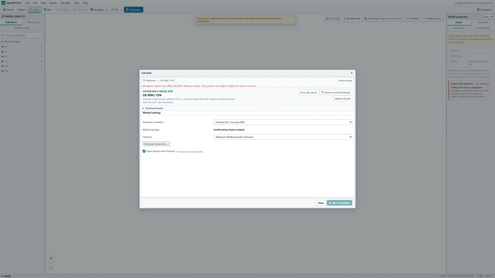
CB-SEM / CFA settings in QuickPLS. Select your own dataset and model, then use the choices described in the steps.
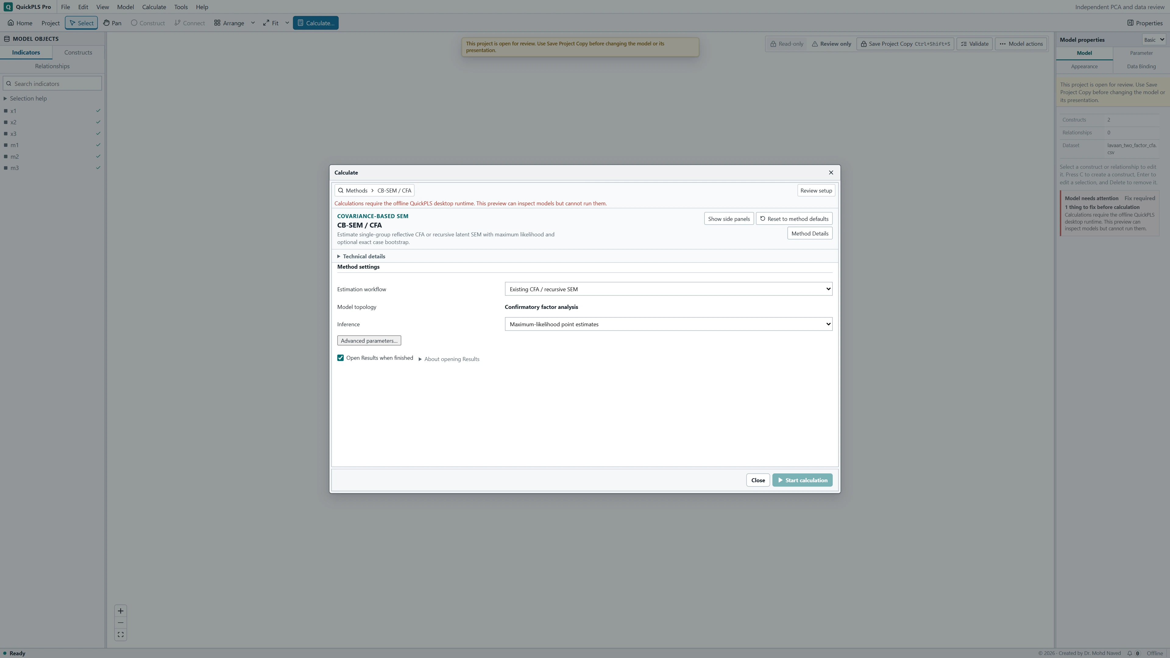
Estimate the covariance-only CFA
Choose the saved CFA
Open Calculate… and choose CB-SEM / CFA. Confirm the workshop dataset and saved CFA. Set Estimation workflow to Existing CFA / recursive SEM and check that Model topology reads Confirmatory factor analysis. A structural topology at this point means that a directed factor relationship remains in the model.
What you should see: Model topology identifies Confirmatory factor analysis for the saved CFA.
How to read it: If it names a structural model, inspect the factor relationships before continuing.
Use maximum-likelihood point estimates
Set Inference to Maximum-likelihood point estimates. This estimates the CFA parameters before optional bootstrap inference. The starting CFA uses the covariance structure; there is no Moment structure selector in this workflow. Leave authored constraints, parameter formulas and structural-effect inference out of the first analysis. Review Readiness, keep Open Results when finished selected and click Start calculation.
What you should see: A separate maximum-likelihood CFA result is saved.
How to read it: Assess that measurement model before fitting the structural extension.
Review the result before interpreting it
After calculation, check convergence, warnings and the usable case count. Then inspect the parameter estimates, residual variances, factor correlations, fit indices and covariance residuals. A completed calculation alone does not establish that the model is suitable.
What you should see: The completed output includes convergence, case count, parameters and fit diagnostics.
How to read it: Investigate negative residual variances, inadmissible correlations or large residuals before interpreting the factors.
Read the parameter and fit tables together
Begin with convergence and admissibility. The optimiser must reach a solution, and estimated variances must make statistical sense. A negative residual variance or an invalid factor covariance matrix requires investigation before interpreting loadings or structural coefficients.
Unstandardized estimates use the units established by the marker indicators. Factor-standardized estimates, labelled std_lv, standardize the factors. Fully standardized estimates, labelled std_all, also standardize the observed variables. Compare coefficients only after confirming which column and scaling convention you are reading.
A freely estimated loading should be accompanied by its available standard error or confidence interval. A fixed marker loading has a different role: its value is imposed to establish the factor scale, so it is not tested as a freely estimated parameter.
Overall fit indices summarize how well the model reproduces the observed covariance relationships. Read them with the model’s degrees of freedom and the residual table. A small set of acceptable summary indices can still conceal a concentrated pattern of unexplained relationships.
In Results, select Workshop CFA in the Result dropdown. Use Search result outputs to find Model parameters or CB-SEM parameter table, Standardized parameters, Model fit or CB-SEM model fit, and Residual covariance. Read the table title and scale before comparing fixed markers, estimated loadings and fit.
On a small screen, swipe the table sideways to see every column.
| Output | How to read it | What to check |
|---|---|---|
| Unstandardized / standardized estimates | Parameters on the declared scale and their standardized counterparts. | A change in scaling can alter coefficients without changing the underlying fit. |
| Fit indices and residuals | Different summaries and locations of model discrepancy. | Check degrees of freedom and definitions rather than collecting cutoffs. |
| Convergence / admissibility | Whether an interpretable solution was obtained. | Investigate invalid variances or nonconvergence before drawing conclusions. |

What the CFA specifies
The CFA assigns each observed indicator to a factor, fixes the factor units through named markers, and estimates factor covariances and indicator residual variances. Cross-loadings and residual covariances are absent from this workshop model. Adding either changes the measurement hypothesis and requires an explanation tied to the indicators, not simply a better fit statistic.
Interpret loadings, factor correlations and residuals
The marker loading fixed to 1 defines the factor’s unit. Its indicator still has a residual variance. For the remaining indicators, inspect the estimated loadings and their uncertainty, keeping unstandardized and standardized columns distinct.
For illustration, fully standardized loadings of 0.80, 0.70 and 0.90 would indicate positive relationships of different strengths with the factor. These values are hypothetical, not workshop estimates. Do not judge a factor from its largest loading while ignoring weak indicators, unexplained covariance or problematic residual variances.
Factor correlations address whether the proposed factors are empirically distinguishable. Very high correlations require attention to item content, the uncertainty of the estimates and competing explanations. They do not by themselves justify merging factors.
A covariance residual is a relationship that the model has not reproduced. Inspect patterns across indicators rather than releasing a covariance for every large residual. A plausible wording or measurement explanation should precede any revised model.
Degrees of freedom describe the model’s restrictions relative to the information available. A just-identified model has zero degrees of freedom and reproduces the analysed moments by construction; its exact fit cannot provide an overall test of the proposed structure.
On a small screen, swipe the table sideways to see every column.
| Output | What to read | Example or warning |
|---|---|---|
| Loadings | Fixed marker, free estimates and standardized metric | A marker fixed at 1 establishes scale. |
| Factor covariances or correlations | Distinctness and the specified relationships | An inadmissible relationship requires investigation. |
| Residual variances | Variation not represented by the factors | A negative variance is not a desirable improvement. |
| Standard errors and intervals | Precision for the parameter on its stated scale | Fixed parameters do not have ordinary estimated uncertainty. |
| Fit and residuals | Global discrepancy and local misfit | A good single index does not validate every loading. |
| Convergence diagnostics | Whether the numerical solution is usable | Check the convergence result even when the screen displays estimates. |
Diagnose a problematic fit
First check the data and the model actually fitted. Indicator assignments, marker choices, covariance roles and unintended restrictions can explain an apparent numerical problem. Retain the initial model and output before making a correction.
After correcting a genuine error, refit and document the change. When the specification is intentional, weak or conflicting evidence is a result to explain. Do not conceal it by reporting only selected indices or the most favourable model.
On a small screen, swipe the table sideways to see every column.
| Symptom | Check | Reasonable action |
|---|---|---|
| A residual variance is negative | Identification, indicator overlap and model assumptions | Investigate an improper solution before reporting fit or paths. |
| A factor loading is fixed at 1 with no ordinary error | Marker identification | Describe it as a scale-setting parameter, not perfect measurement. |
| Fit improves after many residual covariances | Whether each covariance has a substantive reason | Separate exploratory revisions from the original confirmatory specification. |
| A matrix result disagrees with raw data | Cases, variable order, denominator, scales and means | Match the actual inputs before judging the estimator. |
| Improved convergence is unavailable | Whether the analysis includes constraints, formulas or inference | Use the supported procedure and report its scope accurately. |
| Bootstrap or effect intervals are unavailable | Failed fits and expression-specific eligibility | Report the reason; do not replace the result with an unrelated interval. |
Make a justified revision
A revision should address an identifiable problem: an incorrectly coded item, a defensible wording-related residual relationship, or a theoretically distinct factor model. State the reason before fitting the alternative, and consider how the change affects the meaning and coverage of the construct.
Keep the original and revised models, their estimates, fit and warnings. Explain whether the substantive interpretation changes, rather than reporting only the improvement in a fit statistic. A data-driven revision should be described as such.
The exercise treats the indicators as continuous. It does not demonstrate WLSMV, an estimator used for ordinal indicators, multilevel sampling or a robust correction for every form of non-normality. Choose an analysis appropriate to the actual measurement and sampling design.
From correlated factors to a structural model
The CFA allows every pair of factors to covary. A structural model explains some of those relationships through directed paths. It must therefore be specified separately: retaining all six CFA covariances alongside the directed paths would not produce the intended model.
For this extension, Quality and Trust are exogenous factors, meaning that no other factor predicts them. Their covariance remains free. Satisfaction and Loyalty are predicted factors, each with a disturbance variance representing variation unexplained by its predictors. Do not add disturbance covariances to the baseline exercise.
Fit the separate structural extension
Use the same data, indicator assignments and marker loadings as the CFA. Keeping these choices fixed makes the change in structural assumptions clear. The following specification uses covariances only; it does not estimate observed intercepts or factor means.
The Numerical solver panel controls how the calculation searches for parameter estimates. Convergence tolerance and Maximum iterations per stage concern numerical stopping, not the strength of the model’s evidence. Record their values. Do not loosen a tolerance merely to obtain a result that looks more favourable.
When diagnosing a calculation, read the objective, gradient and iteration information with the model warnings. More iterations cannot repair a singular dataset, an unidentified parameter or a substantively incorrect model. If an eligible alternative solver is used as a sensitivity check, retain both results and explain any difference.
For a separate analysis that explicitly models means, the structural workflow offers Moment structure: Covariances and means. It also requires identified observed-intercept and factor-mean specifications. Changing the selector alone does not define those assumptions; keep this extension separate from the covariance-only workshop analysis.
Create a separately named model
Create a separate model named, for example, Workshop structural model. Reproduce the four common factors, their twelve indicators and the same four marker choices. Keep the CFA model and its result intact.
What you should see: A separately named structural model contains the same factor blocks and markers.
How to read it: The original CFA remains available for comparison.
Specify the research paths
Add Quality → Satisfaction, Trust → Satisfaction and Satisfaction → Loyalty as structural paths. Add only the Quality–Trust factor covariance, using Relationship type: Covariance and Relationship use: Model covariance, then Apply relationship use. Do not reproduce the other five CFA covariances. Keep cross-loadings, residual/error covariances and disturbance covariances absent.
What you should see: Three directional paths and the Quality to Trust covariance define the structural model.
How to read it: The other five CFA covariances should not remain as unintended free relationships.
Select the structural estimation workflow
Open Calculate… > CB-SEM / CFA. Set Estimation workflow to Continuous-linear structural ML, Moment structure to Covariances and Inference to Maximum-likelihood point estimates. Model topology should identify a Continuous-linear structural equation model. Leave authored constraints, parameter formulas and structural-effect inference out of this first structural fit.
What you should see: The selected workflow identifies a continuous-linear structural equation model.
How to read it: Confirm Covariances and point estimation before choosing the solver.
Review the solver and results
Open Numerical solver and use Solver: Improved convergence when offered for this specification. Record Convergence tolerance and Maximum iterations per stage, then calculate. Inspect convergence, admissibility, measurement estimates, structural paths and residual fit before reporting any relationship.
What you should see: The structural result records solver settings, convergence and parameter estimates.
How to read it: Assess admissibility and residual fit before interpreting the path coefficients.
Write the method and results
Methods wording to adapt: “We specified a four-factor reflective CFA for Quality, Trust, Satisfaction and Loyalty, each measured by three indicators. The loading of the first named indicator of each factor was fixed to 1. All six factor covariances were estimated; cross-loadings and residual covariances were absent. The covariance-only model was estimated by ordinary maximum likelihood. A separate structural model specified Quality and Trust as predictors of Satisfaction, Satisfaction as a predictor of Loyalty, and a covariance between Quality and Trust.” Add the actual usable sample, software version, calculation settings and any departures from this specification.
For an optional bootstrap analysis, report the requested and usable refits, failures, confidence level, interval method, alternative and seed. For any model revision, report the substantive reason and retain enough detail to reconstruct both models.
Hypothetical results wording for the optional mediation extension: “The Quality → Satisfaction and Satisfaction → Loyalty coefficients were 0.50 and 0.40. Their product was an indirect effect of 0.20. With a direct effect of 0.10, the total effect was 0.30.” Replace these illustrative values with your actual estimates and their matching uncertainty, and report measurement quality, fit and admissibility alongside them.
| Report item | Include |
|---|---|
| Data | Analysed sample, indicator scale and missing-data rule |
| Identification | Markers or other supported factor scaling |
| Measurement | Loadings, covariances, residual variances and fit |
| Structure | Paths and supported effects with their own intervals |
| Restrictions | Exact equality/fixed constraints and defined formulas |
| Numerical procedure | Solver, completion diagnostics and bootstrap settings |
| Sensitivity | Original and revised models with reasons for changes |
Keep a reproducible analysis record
- Save the dataset description, indicator assignments, marker choices, covariance and path specifications, calculation settings and complete results with the report.
- Use the reporting table above as the main checklist. If you report an optional matrix, constraint or effect analysis, include the additional conventions needed to reconstruct it.
Check your analysis
- Identify the four fixed marker loadings and explain why fixing a loading to 1 does not remove its indicator’s residual variance.
- Locate every factor covariance in the CFA, then explain why only the Quality–Trust covariance remains in the specified structural extension.
- Read a freely estimated loading, its uncertainty and a factor correlation. Check for invalid variances or concentrated covariance residuals before interpreting them.
- Record the estimator, covariance or mean convention and numerical settings; for bootstrap results, record the requested and usable refits and interval settings.
- Distinguish an equality restriction from a derived parameter. If using matrix input, document its sample size, variable order and denominator.
- For the optional indirect effect, identify the named paths and the interval that belongs to their product.
Scope of the exercise
This is a continuous, unweighted, single-group maximum-likelihood exercise. It supplies a complete model specification and interpretation guidance, not a newly executed workshop analysis. The saved captures and benchmark comparisons have their own models and versions.
Improved convergence is available for eligible point-estimation models. Constraints, parameter formulas, bootstrap inference and structural-effect inference have their own supported calculations and restrictions. Check the settings offered for the saved model rather than assuming that every option can be combined.
Optional methods and settings
What case-resampling bootstrap intervals add
A case-resampling bootstrap repeatedly draws complete rows with replacement and refits the specified model. The variation across usable refits is used to estimate uncertainty. Keep the model, preprocessing and parameter definitions fixed across these refits.
The available interval methods depend on the chosen calculation. Percentile intervals use ordered bootstrap estimates; BCa intervals adjust for bias and acceleration; analytic studentized intervals also use standard-error information. Where the app offers these choices, record the exact method rather than reporting only that a bootstrap was used.
Intervals labelled Type 7 use that quantile convention to select endpoints. Requested refits and usable refits are different counts. Report failures and exclusions alongside the interval settings.
Request and assess bootstrap inference
Complete a valid point fit before requesting bootstrap intervals. Repeatedly fitting an inadmissible model does not resolve the underlying problem. With raw data, confirm the usable rows after listwise deletion; all twelve workshop indicators are complete, but other datasets may lose cases.
For this teaching exercise, request 1000 bootstrap samples. This is a proposed setting, not a completed workshop calculation. Record the confidence level, interval method, alternative and seed actually used. Keep a two-sided test unless the research hypothesis and analysis plan justify a directional alternative.
Inspect the usable and failed refit counts. A substantial pattern of failed or inadmissible refits can signal unstable identification, unusual observations or a model that is difficult to estimate in smaller effective resamples. Diagnose the cause before interpreting a narrow interval.
Use the interval for the parameter or effect being reported. An interval for a single structural path is not an interval for an indirect effect, which depends on several estimated paths. A result does not acquire effect-specific uncertainty simply because other parameters have bootstrap intervals.
Choose bootstrap inference for the saved model
Open Calculate… > CB-SEM / CFA with the intended model and dataset. Set Inference to Case-resampling bootstrap and Bootstrap samples to 1000. Confirm the model and data remain eligible for the selected procedure.
What you should see: Case-resampling bootstrap is selected for the intended saved model.
How to read it: The 1,000 draws are a teaching choice; retain the final draw count used for your study.
Record the offered interval settings
Set Confidence level (%) and Seed. Where Interval method and Alternative are offered, select and record their exact values, such as Percentile (Type 7) and Two-sided. If the selected calculation fixes these choices, record the stated choices instead of looking for unavailable controls.
What you should see: The requested or fixed confidence level, interval method, tail rule and seed are recorded.
How to read it: Use the interval name actually returned by the calculation.
Inspect usable refits before reporting intervals
Review Readiness and click Start calculation for the selected bootstrap settings. In the completed result, retain the requested count, usable count, failures and any exclusions. Check which parameters or effects received intervals. Save these results with their model and calculation settings so the analysis can be repeated.
What you should see: The result states requested and usable refits and the parameters with intervals.
How to read it: Investigate failures and report the usable count with the intervals.
When the input is a covariance or correlation matrix
A matrix can contain enough information for some covariance-based analyses, but the matrix alone is not a complete specification. You also need its variable order, sample size and denominator convention, together with means or standard deviations when required by the intended analysis.
Use the original sample size. Changing it changes inferential calculations; it is not a way to improve fit. A matrix has no individual rows to resample, so the raw-data case bootstrap is unavailable for matrix-only input.
Check matrix conventions before comparing results
In Project dataset, select the intended matrix dataset and verify that its variable order matches the model’s indicators. Check Covariance denominator for a covariance matrix. For a correlation matrix, review Correlation scales and provide the required standard deviations if the analysis needs the original units. Provide means only for a supported mean-structure analysis.
A covariance of 0.50 and a correlation of 0.50 are not interchangeable. Covariance depends on the units of both variables; correlation removes those units. Substituting one matrix for the other without the corresponding scaling information changes the analysis.
As a hypothetical denominator example, a covariance matrix calculated with N = 100 uses a denominator of 100, whereas a sample covariance calculated with N − 1 uses 99. Multiplying the latter by 99/100 converts it to the former. Confirm the actual convention before converting a supplied matrix.
Check symmetry, diagonal values and sample size before fitting. Keep the same indicator order, scaling, means and likelihood conventions when comparing matrix and raw-data results. Do not attach a case-resampling interpretation to a matrix-only analysis.
Comparing estimates and fit across software
A comparison is meaningful only when both analyses use the same data and model definitions. Match factor scaling, covariance denominators, means, parameter counts and the likelihood definition before interpreting a difference in coefficients or fit criteria.
Use the linked numerical evidence pages for their specific checked models and quantities. Their results do not supply fitted answers for this workshop.
Illustrative example, not a software benchmark
Two programs agree on loadings but report slightly different information criteria. First align the likelihood constant, covariance divisor and parameter count. A difference may follow from a documented convention rather than an optimisation error. The CFA benchmark record illustrates such an alignment.
Restrictions and calculated quantities
A constraint restricts parameters that the model estimates, such as requiring two loadings to be equal. A defined parameter calculates a quantity from fitted parameters, such as an indirect effect a × b. A restriction can change the fit; a calculated quantity does not by itself add a restriction.
Specify the hypothesis, parameter labels and formula before fitting. Keep fixed, free, constrained and derived quantities distinct. An intended comparison is interpretable only if the model remains identified and the chosen calculation supports the restriction.
Specify a restriction or derived effect
The examples in the table show different operations. Requiring two loadings to be equal limits the fitted measurement model. Fixing Quality → Loyalty to zero limits the structural model. Calculating an indirect or total effect summarizes estimates from an already specified model.
Save the unrestricted model before imposing a restriction. Record the exact parameters involved, their fixed or free roles and the reason for the restriction. A marker loading already fixed to 1 is not an ordinary free loading that can be released or tested in the same way.
For a nested model comparison, confirm that the models use the same data, variables, estimator and compatible likelihood definition. The more restricted model must be obtainable by imposing the stated restrictions on the less restricted model. A change in fit alone cannot establish the substantive reason for a restriction.
For the zero-path comparison, retain the unrestricted model and use the separate CB-SEM Model Comparison workflow after saving the restricted model. Check the intended parameter restriction and shared dataset before interpreting the comparison.
On a small screen, swipe the table sideways to see every column.
| Specification | What it does | How to report it |
|---|---|---|
| Two loadings constrained equal | Restricts the fitted parameter space | Name both loadings and state the equality. |
| Quality to Loyalty fixed at zero | Imposes a structural restriction | Explain the hypothesis and compatible comparison. |
| Indirect = a × b | Defines a function of estimated paths | Name the path and its supported uncertainty. |
| Total = direct + indirect | Summarizes a stated set of effects | List the included direct and indirect terms. |
Specify the effect you intend to report
A direct effect follows a specified structural path. An indirect effect follows a route through one or more mediators. A total effect combines the relevant direct and indirect routes. Name the starting variable, outcome and intervening paths before interpreting the result.
If comparing effects, state the exact contrast and its uncertainty calculation. Statistical evidence for an effect does not establish a causal explanation without an appropriate design and assumptions.
An indirect-effect calculation
As an optional extension, add Quality → Loyalty to a separately named structural model while retaining Quality → Satisfaction → Loyalty. This distinguishes a direct Quality–Loyalty relationship from the route through Satisfaction.
For a hypothetical example, let Quality → Satisfaction be a = 0.50 and Satisfaction → Loyalty be b = 0.40. The indirect effect is a × b = 0.20. If the direct effect is 0.10, the total effect is 0.30. These are arithmetic examples, not estimates from the workshop data.
The uncertainty of a × b depends on the joint behaviour of the two path estimates. Multiplying their separate confidence-interval endpoints does not produce an indirect-effect interval. For the saved structural extension, open Calculate… → CB-SEM / CFA with Continuous-linear structural ML. Under Structural effects choose Effects with normal-delta inference for the point workflow, or Effects with bootstrap inference after selecting Case-resampling bootstrap. Expand Requested effects and path limit, click Add requested effect and set Effect type to Specific indirect path. Set Path step 1 to Quality → Satisfaction and Path step 2 to Satisfaction → Loyalty. Record the offered confidence and alternative settings, calculate, and report the named indirect effect with its own interval.
When the model contains several indirect routes, identify each route and explain which are included in a reported total. Positive and negative routes can offset one another. The synthetic, cross-sectional exercise does not establish a temporal or causal mediation mechanism.