 QuickPLS
What the method does
Blindfolding systematically omits selected data entries and uses the fitted model to reconstruct them. Its Q² statistic compares reconstruction errors with a reference sum of squares. It describes the specified omission exercise, which differs from testing predictions on genuinely new cases.
Q² = 1 − SSE / SSO.
SSE is the sum of squared reconstruction errors and SSO is the reference sum of squares for the omitted observations. A positive value means improvement over that reference in this exercise. Report the omission distance and eligible indicators.
Data and analysis in QuickPLS
Use a suitable PLS model and its case-level indicators. Choose an eligible omission distance and examine the app’s case and indicator checks.
QuickPLS runs the blindfolding calculation and reports the eligible redundancy results. Use PLSpredict when the research question concerns performance on held-out cases.
Follow a worked example
The following example shows the data, settings and decisions for one analysis. Use the linked practice files to follow it. For your own study, keep the procedure and choose the variables, model and settings that fit your research question.
Download research-workshop.csv to begin. It contains 360 rows and 31 columns. The example below identifies the variables to use, their roles and any rows to exclude; not every column is an analysis variable.
Blindfolding Q²: reconstruction of omitted values
Blindfolding omits selected indicator values and uses the model to reconstruct them. Repeating this procedure across the dataset gives an error total. The Stone-Geisser Q² statistic compares that error with a reference total.
This is useful when a paper calls for an omission-based, or Stone-Geisser, Q² assessment. It works with reflective outcome constructs: groups of indicators that reflect an underlying concept, where another construct in the model predicts that concept. It reuses the same people’s data. To ask how well the model predicts people left out of fitting, use the PLSpredict/CVPAT guide.
The omission distance controls the pattern of cells left out. Whether a distance is valid depends on the number of usable cases. Check that number before calculating; the value shown by default is not a substitute for checking the sample.
Practice with the Satisfaction and Loyalty model
Download research-workshop.csv and the data guide below. The file has 360 synthetic cases. Use Quality, Trust, Satisfaction and Loyalty, with their three matching indicators, and draw Quality → Satisfaction, Trust → Satisfaction and Satisfaction → Loyalty.
The arrows make Satisfaction and Loyalty endogenous constructs: outcomes explained by something else in the model. Quality and Trust are exogenous constructs here: they have no incoming arrows. Being measured by indicators does not make an exogenous construct eligible for this redundancy Q² assessment.
In this lesson you will choose a valid omission distance, find the error totals and explain the resulting ratio. The exercise illustrates the omission-based Stone-Geisser assessment found in older studies. The numerical examples below are separate teaching examples; this page does not give a checked Q² answer for the practice CSV.
Check the outcomes and the usable rows
In the workshop model, arrows run from Quality and Trust to Satisfaction, then from Satisfaction to Loyalty. Satisfaction and Loyalty are the outcomes to assess. Quality and Trust have no incoming arrows in this model, so they are outside this outcome-redundancy calculation.
Check that the outcome constructs use Reflective measurement. Then record how many cases the calculation will actually use after any missing-data exclusions. Keep the row order, indicator order and model settings if you need to reproduce a previous study. These details determine the omission exercise.
Omission-distance rules and output labels
Use the saved workshop model and check its analysed sample before choosing Omission distance. The complete file has 360 cases; missing-data exclusions in another file can change which distances are valid.
Set Omission distance. The panel accepts distances from 5 to 12, but the chosen value must also be smaller than the analysed sample and must not divide that sample size exactly. Read Readiness before running; a number within the field’s range can still be invalid for your data.
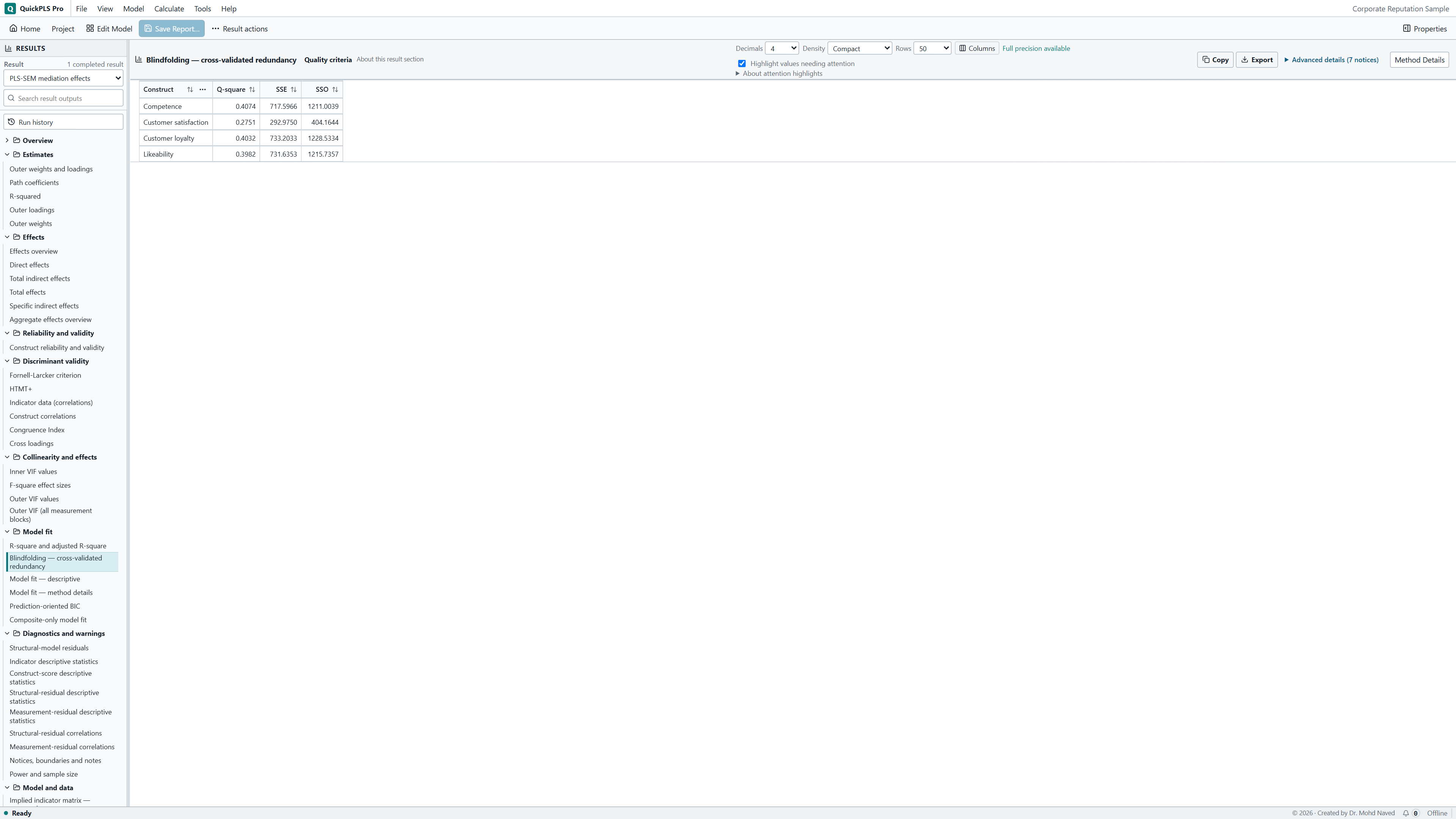
Keep Open Results when finished selected and click Start calculation. In Results, check the selected run in the Result dropdown. Open Model fit → Blindfolding — cross-validated redundancy, or type Blindfolding in Search result outputs. Read each eligible construct’s Q-square, SSE and SSO. Some result views use Q², Prediction error and Observation sum for those columns; the error total is the quantity called PRESS in this guide.
Run the omission exercise step by step
Check the model’s analysed sample
Run the ordinary PLS analysis first and record the number of cases actually used. Confirm the reflective Satisfaction and Loyalty constructs. If missing-data treatment removes rows, use the remaining count when checking the omission distance.
What you should see: The analysed sample count and required indicators are known.
How to read it: The omission plan must suit that sample.
Open the calculation
Click Calculate…, enter Blindfolding (Q²) in Find a method and select it. Check that this is the intended model. Keep the source rows and indicators in the same order when reproducing an earlier result.
What you should see: Blindfolding is selected for the intended model.
How to read it: Keep this result separate from held-out prediction.

Blindfolding (Q²) settings in QuickPLS. Select your own dataset and model, then use the choices described in the steps. Set Omission distance to 7
For 360 analysed cases, 7 is smaller than the sample and does not divide it exactly. A distance of 5 divides 360 and is invalid for this rule. Omission distance describes a pattern of missing cells; it is not the number of cross-validation folds used by PLSpredict.
What you should see: Omission distance is 7 for this practice run.
How to read it: Confirm the app accepts that distance for the analysed data.
Review the settings and run
Check Weighting scheme and the readiness message. Advanced settings contains Maximum iterations and Stop criterion if you need to reproduce recorded settings; do not change them simply to seek a larger Q². Click Start calculation and allow the complete procedure to finish. In each omission round, the means of the remaining training values fill the omitted cells before the model is refitted. This preparation is part of blindfolding; it is not a general recommendation for replacing missing research data.
What you should see: The saved calculation records its omission settings.
How to read it: An incomplete reconstruction does not supply an interpretable Q².
Inspect the complete result
Open Model fit → Blindfolding — cross-validated redundancy. You can also find it with Search result outputs. For each eligible construct, read the error total (SSE or Prediction error, called PRESS here), SSO and Q². Check warnings and unavailable reasons before interpreting the ratio. Save the sample count, distance, row and indicator order and estimation settings with the result.
What you should see: The result identifies eligible redundancy values and their components.
How to read it: Interpret Q² as omission-based relevance, then use held-out prediction for a new-case question.

Error totals and Q²
PRESS is the sum of squared errors when reconstructing the omitted answers. A larger error makes the total larger. The app may label this column SSE or Prediction error. SSO, also shown as Observation sum, supplies the reference total used in this calculation.
Q² puts those totals together as 1 − PRESS/SSO. A positive value means the reconstruction error is below the reference total. A negative value means it is above the reference total. If SSO is zero or invalid, the ratio is unavailable; a blank value is not evidence of perfect performance.
Read the rows for each eligible construct and inspect any warning or unavailable reason. These are errors from omitted cells in this procedure. They are not the errors for new cases in a PLSpredict test.
On a small screen, swipe the table sideways to see every column.
| Output | How to read it | What to check |
|---|---|---|
| SSO | Reference sum of squared observations under the procedure. | A zero or invalid denominator makes the ratio unavailable. |
| PRESS | Prediction-error sum from the declared omission procedure. | It is not the same error produced by held-out PLSpredict folds. |
| Q² | 1 − PRESS/SSO for the specified redundancy calculation. | Interpret it as reconstruction under this omission procedure, not accuracy for new cases. |
Work through positive, negative and unavailable Q²
Take a hypothetical error total, PRESS, of 120 and a reference total, SSO, of 200. The calculation is 1 minus 120 divided by 200, giving Q² = 0.40. Reconstruction has less error than the reference under this omission procedure.
Now keep SSO at 200 but let PRESS be 260. Q² becomes -0.30. This is a valid negative result: reconstruction is worse than the reference. Report the sign. Replacing it with zero would change the finding.
If SSO is zero, division by that total is undefined. The appropriate result is unavailable. Check whether the relevant data have variation and read the calculation’s reason before trying to interpret it.
These numbers illustrate the ratio; they are not results from research-workshop.csv. Inspect the available construct and indicator details, since an aggregate result can conceal uneven reconstruction.
Keep blindfolding Q² separate from Q²_predict. The latter belongs to held-out prediction and uses a different procedure and reference. Similar names, or two positive numbers, do not make the two results interchangeable.
Invalid settings and negative Q²
First decide whether you have an invalid calculation or an interpretable weak result. An invalid distance needs correction. A negative Q² is a finding to understand. Use the table to choose the next check without changing the sample or settings just to improve the number.
On a small screen, swipe the table sideways to see every column.
| Symptom | Check | Reasonable action |
|---|---|---|
| The omission distance is rejected | Check that it is smaller than the analysed sample and does not divide that sample size. | Choose a valid supported distance and record it. Do not alter the sample solely to make a preferred distance valid. |
| An exogenous or formative construct has no Q-square | Check its role and measurement type. | Report it as outside this redundancy assessment. Do not reinterpret an absent value as zero predictive relevance. |
| Q-square is negative | Inspect PRESS relative to SSO and review the measurement and structural specification. | Describe worse reconstruction than the benchmark. Investigate the model rather than suppressing the sign. |
| A construct is unavailable | Check zero benchmark variation, nonfinite values or failed nested estimation. | Retain the reason and resolve a genuine data or estimation problem. Do not average only successful rounds. |
| A reproduced value differs from an older run | Compare the analysed sample, row order, indicator order, omission distance and estimation settings. | Align the actual procedure before attributing the difference to software. A shared method name alone is insufficient. |
Check whether an older result can be reproduced
If your study needs a sensitivity check, plan another valid omission distance and retain the same sample, model and ordering. Then compare both results. If the sign or size changes substantially, explain that dependence instead of choosing the better-looking value.
With the same recorded schedule, blindfolding is deterministic: it repeats the same omission exercise. Trying many row orders to find a favourable result is not a useful check of robustness.
For a new prediction question, use a validation design suited to the people, setting and timing of the intended prediction. A model can reconstruct omitted cells reasonably yet add little value for held-out cases. Report that difference as a difference between research questions, not as a contradiction or a relabelled replication.
Methods and results example
After completing this practice run, a methods paragraph could say: “We assessed the reflective outcome constructs with omission-based Stone-Geisser redundancy analysis. The analysis used 360 complete practice cases and omission distance 7. We kept the recorded row and indicator order. In each omission round, we filled the omitted cells with the means of the remaining training values before refitting the model.” Use this wording only when it describes the run you performed.
For the separate arithmetic example, a results paragraph could say: “PRESS was 120 and SSO was 200, giving Q² = 0.40 for the illustrated construct. Reconstruction error was below the reference total under this omission procedure.” Add that this is an omission-based diagnostic. It is not evidence of out-of-sample predictive power.
In your paper, substitute the actual construct names and values, include failed or unavailable calculations and state the error-column label used in the export. Give any held-out prediction results their own paragraph. The table lists what another researcher needs to repeat the analysis.
| Field | Report |
|---|---|
| Purpose | Historical replication or descriptive redundancy question. |
| Eligibility | Endogenous reflective constructs and analysed sample. |
| Schedule | Omission distance, row/indicator order and preparation rule. |
| Results | PRESS, SSO, Q-square and unavailable or failed calculations. |
| Interpretation limit | Explicit distinction from PLSpredict, CVPAT and external prediction. |
What to keep for your paper
- Name the reflective outcomes assessed and state how many cases the calculation used.
- Record Omission distance, the row and indicator order, and the model’s estimation settings.
- Report the error total, SSO and Q² together. Explain whether you use PRESS, SSE or Prediction error for the error total so readers can match your report to the exported table.
- Keep warnings, failed rounds and unavailable values with their reasons. If your paper also makes a claim about prediction for new cases, report that separate assessment.
Choose the right result for your research question
A positive blindfolding Q² supports a statement about reconstruction within the recorded omission exercise. It does not show how accurately the model predicts a new customer or a future observation.
For a prediction claim, continue to PLSpredict or CVPAT and define which information would be available when making the prediction. You can report both assessments when the study needs them, but give each its own name, procedure and conclusion.
Check that you can explain your result
- Show why 7 is a valid distance for 360 cases and why 5 is not.
- Identify Satisfaction and Loyalty as the eligible reflective outcomes in the starting model, and explain why Quality and Trust are excluded from this assessment.
- Find the error total and SSO in the app, and use them to reproduce both the positive and negative teaching examples.
- Explain why zero SSO makes the ratio unavailable rather than perfect.
- Describe what the result says about reconstruction, then name the separate assessment needed for a claim about prediction for new cases.
Optional methods and settings
Additional arithmetic example
The numbers below show how the ratio works. They are an arithmetic example, not an answer you should expect from the workshop data.
Illustrative example, not a software benchmark
With illustrative SSO = 100 and PRESS = 70, Q² = 0.30. The omission-based error is below its reference sum. This calculation does not show that the model would outperform a simple linear model when predicting future cases.