 QuickPLS
What the method does
Weighted PLS uses a declared weight for each case in data summaries and model estimation. Weights may represent a documented sampling or adjustment scheme. They alter the population summary being estimated; they are not indicator weights and should not be chosen to make relationships stronger.
Weighted mean: x̄w = Σᵢwᵢxᵢ / Σᵢwᵢ. Weight concentration: n_eff = (Σᵢwᵢ)² / Σᵢwᵢ².
The case weight wᵢ controls the contribution of observation xᵢ. The effective sample size n_eff describes concentration of the weights; it is not a substitute for a full complex-survey design calculation.
Data and analysis in QuickPLS
Provide the model indicators plus the eligible numeric case-weight column. Inspect missing, zero, negative and very large weights according to the app checks, and document how the weights were constructed.
QuickPLS applies the chosen weight column to your PLS model and provides case-weight diagnostics alongside the model results. You can use your own data after checking the weighting scheme and measurement specification.
Follow a worked example
The following example shows the data, settings and decisions for one analysis. Use the linked practice files to follow it. For your own study, keep the procedure and choose the variables, model and settings that fit your research question.
Download research-workshop.csv to begin. It contains 360 rows and 31 columns. The example below identifies the variables to use, their roles and any rows to exclude; not every column is an analysis variable.
Use a case weight when some rows should contribute more
A case weight controls how much one observation contributes to the calculation. A row with a larger weight has more influence than a row with a smaller weight. This is different from an indicator weight, which is used to combine measurements into a construct score.
Choose weighted PLS when you have a reason for unequal case contributions. Explain whether the weights represent a sampling adjustment, frequency information or another justified rule. The column itself cannot tell the software what that reason is.
Keep the weight column separate from the model's indicators and predictors. A few large weights can concentrate much of the influence in a small part of the dataset, even when the file has many rows.
This procedure fits a weighted reflective PLS model. Reflective indicators are treated as expressions of the concept they measure. A positive weight column alone does not supply the additional corrections required for a complex survey with separately sampled groups or clustered observations.
Practise with deliberately unequal case weights
Use research-workshop.csv with Quality, Trust, Satisfaction and Loyalty as four reflective blocks. Assign their matching indicators and draw Quality → Satisfaction, Trust → Satisfaction and Satisfaction → Loyalty. Select the column named weight through the case-weight control; do not attach it to a construct as an indicator.
Assign quality_1, quality_2 and quality_3 to Quality; trust_1, trust_2 and trust_3 to Trust; satisfaction_1, satisfaction_2 and satisfaction_3 to Satisfaction; and loyalty_1, loyalty_2 and loyalty_3 to Loyalty.
The supplied weights are positive and deliberately unequal so that you can see how different case contributions affect a model. They are teaching values, not validated survey weights. They do not establish that the result represents a particular national or organisational population.
Start with the complete file so you can examine weighting without also changing missing-data preparation. Afterwards, use research-workshop-missing.csv as a separate lesson. Keep both datasets and results.
When a coefficient changes, ask which choice changed with it: case influence, the included sample or the replacement rule. Comparing one choice at a time makes the difference easier to explain.
Check every weight and keep it outside the model
Prepare numeric reflective indicators and a separate weight column. Check for missing values, zero, negative values and nonfinite entries, such as infinity. The selected weights must be positive, finite numbers.
Write down how the weights were created and what one weight unit means. Do this before interpreting a result that changes after weighting.
Select weight under Case-weight variable and confirm that the selected dataset contains this numeric column. Keep it unassigned to every construct. If Readiness rejects the choice, inspect the values before calculating.
Select the weights, preparation rule and calculation
Select the method and the weight column
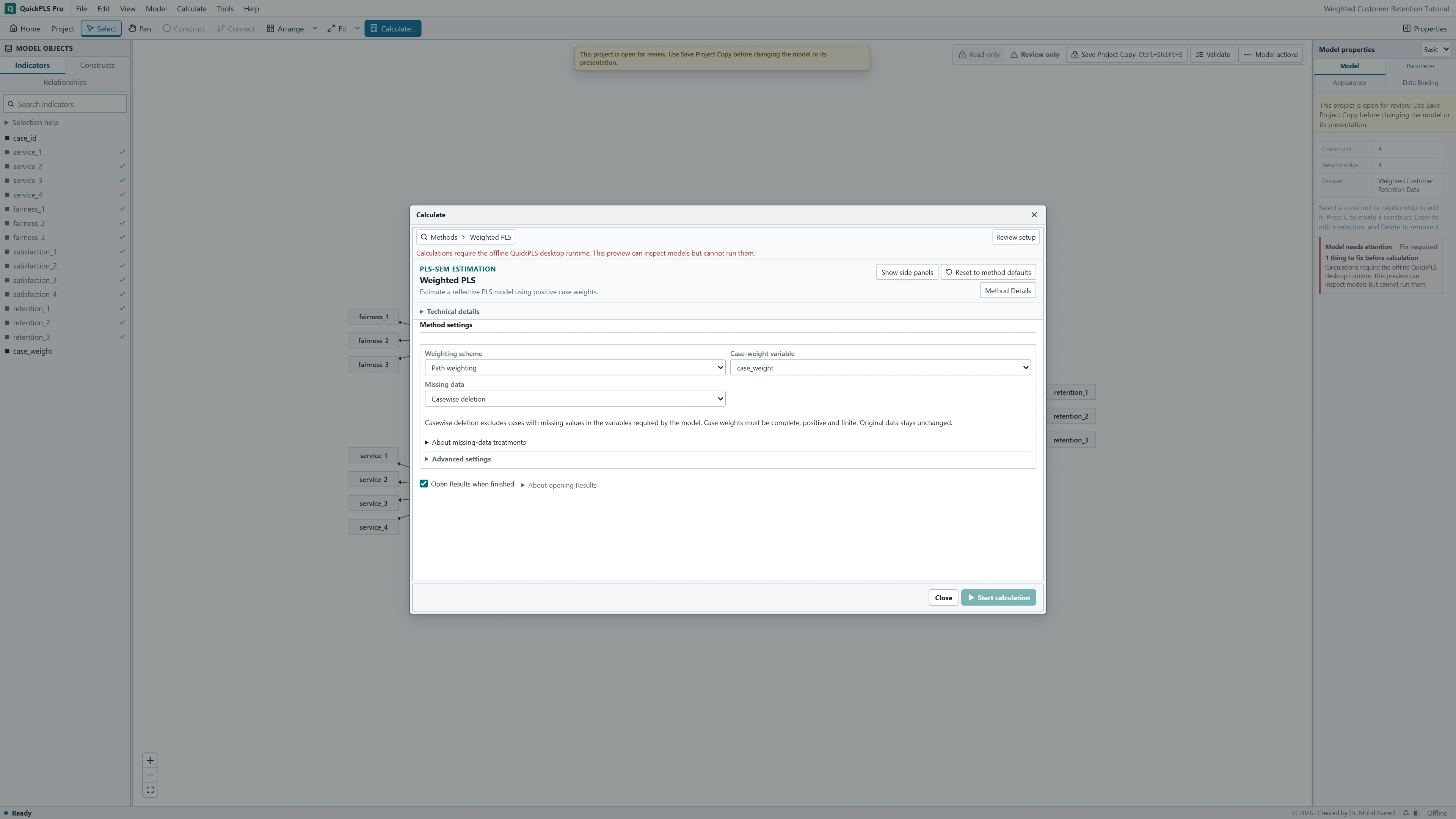
Click Calculate…, type Weighted PLS into Find a method and select that row. Set Case-weight variable to the intended numeric column. For the workshop, choose weight. Check that its values are complete, positive and finite; it must not be attached to a construct as an indicator.
Run the complete-data lesson first
Choose Weighting scheme → Path weighting and Missing data → Casewise deletion for the complete workshop file. Advanced settings contains Maximum iterations and Stop criterion. The ordinary casewise and mean-replacement routes use standardized data without a Result data selector; do not look for a standardization dropdown on this screen.
Use the separate mean-replacement lesson for its bootstrap
For the missing-data lesson, select the intended dataset and model, reselect Case-weight variable, and set Missing data → Mean replacement. This reveals Inference, where Point estimates or Bootstrap can be chosen. Review Readiness, keep Open Results when finished selected, and click Start calculation. Read the weight and preparation checks before interpreting paths.
Run the workshop and check which cases shaped the result
Verify the model and weights
Check the twelve reflective indicators and three starting paths. Keep weight outside the indicator assignments. Inspect weight for complete, positive finite values. Replacing missing indicators will not fill a missing weight.
What you should see: The weight column is separate from the twelve indicators and has valid positive values.
How to read it: Resolve invalid weights before fitting.
Open Weighted PLS and select weight
Click Calculate…, find Weighted PLS, and set Case-weight variable → weight. Choose Weighting scheme → Path weighting. This selector identifies the weight column; it does not select frequency-weight semantics.
What you should see: Case-weight variable shows weight and the chosen weighting scheme is visible.
How to read it: A case weight changes observation contributions, not indicator assignments.
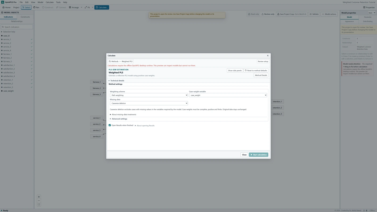
Weighted PLS settings in QuickPLS. Select your own dataset and model, then use the choices described in the steps. Fit the complete-data example
For research-workshop.csv, choose Missing data → Casewise deletion. Expand Advanced settings to inspect Maximum iterations and Stop criterion. Review Readiness, leave Open Results when finished selected and click Start calculation. Keep this result for comparison.
What you should see: A saved complete-data result reports analysed cases and weight diagnostics.
How to read it: Check weight concentration before comparing coefficients.
Prepare the separate missing-data example
Open the model linked to research-workshop-missing.csv, select Weighted PLS and reselect Case-weight variable → weight. Choose Missing data → Mean replacement. Do not merely switch a dataset name while assuming the old model is bound to the new file. Inspect the missing original indicators and the means used to fill them.
What you should see: The second model is linked to research-workshop-missing.csv and Mean replacement is selected.
How to read it: A missing weight still needs its own resolution.
Choose matching uncertainty settings
Under the mean-replacement setup, set Inference → Bootstrap. Record Confidence interval, Confidence level (%), Hypothesis test, Bootstrap draws and Seed. Studentized (nested bootstrap) also reveals Inner draws per sample. Start this as a separate saved result.
What you should see: The separate result records the chosen weighted bootstrap and preparation.
How to read it: Interpret its intervals under that procedure.
Read the correct result tables
Select the intended Result in the Results dropdown. Begin with Diagnostics and warnings → Case-weight diagnostics for mean replacement, then read the preparation information. Open Inference → Weighted bootstrap estimates for its intervals and Weighted mean-replacement bootstrap settings for usable-draw counts. Compare paths only after matching the dataset and preparation.
What you should see: The selected dataset, preparation, weight diagnostics and intervals agree.
How to read it: Compare coefficients only after confirming which calculation each table belongs to.
Check influential weights before interpreting the relationships
Start in Diagnostics and warnings. For the casewise result, open WPLS case-weight diagnostics; the mean-replacement result calls this table Case-weight diagnostics. Read the selected column, Weight sum and Effective sample size. Check the analysed cases and investigate unusually large weights.
Effective sample size summarises how concentrated the weights are. It is different from the number of people or rows in the study. It also does not automatically provide the degrees of freedom used by some tests to determine their reference distribution.
Read weighted loadings and R-square under Estimates. A casewise path table may be labelled Path coefficients; a result with mediation uses Direct effects. The mean-replacement route places Direct effects under Effects. Use Search result outputs if the expected table is not visible, and keep the selected Result on the run you intend to report.
For weighted mean-replacement uncertainty, open Inference → Weighted bootstrap estimates. Read the estimates and their intervals alongside Diagnostics and warnings → Weighted mean-replacement bootstrap settings, which records the requested and usable draws. Interpret them under that saved run's weight definition and preparation.
On a small screen, swipe the table sideways to see every column.
| Output | How to read it | What to check |
|---|---|---|
| Weight totals and eligible rows | Which cases enter the calculation and how much weight each contributes. | Inspect exclusions and extreme weights before the paths. |
| Effective sample size | A summary of how unequal weights concentrate influence. | Do not use effective sample size as the degrees of freedom unless the test defines it that way. |
| Weighted paths and loadings | Estimates under the declared weighting rule. | Use diagnostic measures designed for the selected weighting method. |

A changed coefficient needs a weighting explanation
How to interpret a weighted comparison
Giving a few respondents larger weights can move a path estimate even though the original rows are unchanged. Compare weighted and unweighted results using the same data and preparation, then explain why the weights are appropriate. A large difference by itself cannot identify which estimate best represents the intended population. This is an interpretation example, not a software benchmark.
Report what the weights mean and how they were used
- Identify the source of the case weights and explain what their values represent.
- Report excluded weights or cases, weight totals and the effective-sample information.
- Name the weighted procedure and explain any comparison with an unweighted or modified-weight analysis.
Choose preparation and uncertainty for the intended weight meaning
A case-influence weight increases a row's contribution. A frequency weight represents repeated observations under an explicitly selected procedure. An integer weight can have either intended meaning, so integers alone do not determine the interpretation.
For confidence intervals, the bootstrap repeatedly samples rows and fits the model again. Keep the weight meaning and data preparation inside that procedure. This is how the intervals remain tied to the analysis that produced the estimate.
Choose and explain the case weights
Set Case-weight variable to the intended numeric column and confirm positive, finite values. Record how the weights were created. The ordinary Weighted PLS setup selects a column; it does not offer a separate frequency-versus-case-influence dropdown. Do not interpret integer weights as repeated participants unless the analysis explicitly uses that meaning.
Choose Mean replacement for this lesson
Set Missing data → Mean replacement. This exposes the Inference control used below. The Casewise deletion screen does not show this mean-replacement bootstrap selector. Pairwise deletion has a separate setup and should be followed as its own analysis.
Open and complete the bootstrap controls
Set Inference → Bootstrap. Review Confidence interval, Confidence level (%), Hypothesis test, Bootstrap draws and Seed. Confidence interval offers Percentile, BCa and Studentized (nested bootstrap). The studentized choice also reveals Inner draws per sample. Record these settings before clicking Start calculation.
Read the estimate, interval and usable draws
Open Inference → Weighted bootstrap estimates. Check Diagnostics and warnings → Weighted mean-replacement bootstrap settings for the requested and usable draws. Each resample recomputes the indicator's observed arithmetic mean and retains the sampled row's original weight. Confidence intervals are two-sided; Hypothesis test selects the test direction separately. Read effective sample size under the saved weight definition.
Keep the conclusion within the weighting method used
A positive weight column does not automatically handle clustered sampling or stratification. For example, sampling people together within organisations can affect uncertainty beyond the case weights themselves.
Before applying a rule from an ordinary unweighted analysis, check how the weighted result defines that diagnostic. Report the supported procedure you actually ran, and make the reason for its weighting clear.
Fill an indicator with its arithmetic mean, then fit with weights
In this mean-replacement procedure, the replacement value is the indicator's observed arithmetic mean. If its observed values are 2 and 6 and a third entry is missing, replace that entry with 4. Unequal analysis weights do not turn that replacement into a weighted mean.
Weighted fitting happens after this preparation. Keeping the two operations separate explains why a manual weighted-mean replacement may fail to reproduce the procedure.
The bootstrap also repeats the preparation. Within each raw-case resample, QuickPLS recomputes the arithmetic means from the sampled indicator values, and each sampled row keeps its original weight. Filling the data once and then resampling the completed table would hold the preparation fixed.
Casewise deletion keeps rows complete on every variable required by the model. Pairwise preparation uses the available overlap for each operation and leaves missing cells unfilled. These choices can therefore produce different means, covariances and available scores; they need not use the same information in the same way.
The missing entries in the download are a teaching device. For real data, explain why values are missing and why the chosen preparation is reasonable. Neither mean replacement nor weights by themselves establish that missing-data bias has been resolved.
Distinguish rows, weight totals and effective sample size
Count the actual analysed rows first. Then examine how much of the total weight belongs to a few observations. Effective sample size summarises that concentration under a specified formula; it does not create a new participant count.
For the common case-influence expression, square the sum of the weights and divide it by the sum of their squares. With hypothetical weights 1, 1 and 4, this is 36 / 18 = 2. There are still three rows, but their influence is more concentrated than with equal weights.
Check the exact effective-size definition saved with your QuickPLS result. Frequency weights have a different meaning from case-influence weights, so the same numerical column should not be interpreted under a different definition without changing the stated analysis.
If one weight is very large, inspect its origin and how it affects measurement and paths. A difference from the unweighted result is worth explaining, but does not alone show that the weighted estimate better represents the population.
On a small screen, swipe the table sideways to see every column.
| Output | Hypothetical example or question | Interpretation |
|---|---|---|
| Preparation | Observed values 2 and 6 imply replacement 4 | Arithmetic indicator means precede weighted fitting. |
| Case count | Number of analysed rows | Distinct from sum of weights and effective sample size. |
| Effective sample size | Weights 1, 1, 4 give 2 under the stated expression | A concentration diagnostic, not a new participant count. |
| Weighted measurement and paths | Compare a matched unweighted analysis | Differences reflect the selected weighting definition. |
| Bootstrap intervals | Read selected two-sided bounds | Hypothesis-test direction is chosen separately. |
| Usable draws and failures | Report actual counts | Weights and preparation accompany matching refits. |
Trace an unexpected result to weights, preparation or inference
If weight is absent from Case-weight variable, inspect the active dataset and its column type. The picker lists numeric columns. If Readiness says to choose a positive numeric case-weight variable, select it; if it reports invalid values, check the original column. Mean replacement fills missing indicators, not missing weights.
If the bootstrap fields are absent, check Missing data. The controls described in this lesson appear after Mean replacement → Inference → Bootstrap. Do not add ordinary PLS bootstrapping to a weighted casewise run and describe it as the same procedure.
The table's reference to frequency weighting describes an analysis definition, not an extra dropdown on this ordinary setup screen. Keep the workshop's stated case-influence interpretation. If a path is weak or its interval is wide after the setup is correct, report its estimate and uncertainty; changing weights solely to strengthen it has no research justification.
On a small screen, swipe the table sideways to see every column.
| Symptom | Check | Reasonable action |
|---|---|---|
| Weight column is rejected | Missing, nonfinite, zero or negative entries | Correct genuine errors or define a defensible sample; do not impute weights casually. |
| Effective size is much smaller than row count | Weight concentration and reported definition | Inspect influential weights and their justification. |
| Manual imputation disagrees | Arithmetic indicator mean versus weighted mean | Reproduce the implemented preparation order. |
| Integers were treated as repeated participants | Selected weight interpretation | Use frequency weighting only when explicitly selected and justified. |
| Bootstrap and point conclusions differ | Preparation, weights, interval and test direction | Match settings and read interval and test decisions separately. |
Compare weighting choices one at a time
First compare weighted and unweighted models on the same complete data. Then, under one weight definition, compare the missing-data preparation choices. This sequence helps separate the effect of case influence from the effect of incomplete measurements.
Trace how large weights were calculated. Trimming a weight changes the relative contribution of that case and can change what the analysis estimates. Any trimming rule needs a substantive reason, preferably chosen before inspecting the path of interest.
If trimming is a sensitivity check, keep and report both the original and modified rules and results. Do not present the more favourable estimate as though no alternative was tried.
Complex survey uncertainty may require clustering and stratification information as well as weights. Describe this analysis as the supported case-weighted PLS procedure and explain any design features it does not address.
Write the weighting and preparation clearly
For the teaching model, a Methods description could read: We fitted the four-construct model with the supplied positive case-influence weights. We replaced missing indicator entries with each indicator's observed arithmetic mean before weighted fitting. Raw-case bootstrap refits recomputed those means and kept each sampled row's original weight. We reported the weight definition, row count and effective-size definition separately.
For the arithmetic illustration, a Results sentence could read: Weights of 1, 1 and 4 give an effective sample size of 2 under the stated concentration formula. This sentence explains the formula; it is not the result for the workshop data.
A completed research report needs the actual weighted estimates and intervals, the weight distribution, preparation counts and resampling failures. Explain any matched unweighted comparison and any justified change to the weights.
| Item | Required detail |
|---|---|
| Weights | Column, meaning, positivity checks and distribution |
| Preparation | Casewise, arithmetic mean replacement or pairwise |
| Sample | Actual rows, omissions and effective-size definition |
| Estimates | Weighted loadings, weights, paths and explained variance |
| Inference | Interval, confidence, test direction, draws, seed and failures |
| Sensitivity | Matched unweighted comparison and justified modifications |
Check that you can explain the weighted analysis
- Explain what one unit of the chosen weight represents.
- Confirm that weight was selected as a case weight rather than an indicator.
- Calculate the arithmetic replacement mean for one indicator.
- Distinguish analysed rows, the sum of weights and effective sample size.
- Explain which values are recomputed in each bootstrap resample.
- Explain why the teaching weights do not provide complex-survey uncertainty by themselves.