 QuickPLS
What the method does
A quadratic model includes both a predictor and its square. It can represent a relationship that becomes stronger, flattens or reverses within the data range. The squared coefficient describes curvature, while the linear and squared terms jointly determine the slope and turning point.
Y = b₀ + b₁X + b₂X² + ε; slope = b₁ + 2b₂X; turning point = −b₁/(2b₂), when b₂ ≠ 0.
The turning point has a substantive interpretation only if it lies within a supported range of X. Keep the scale and centering convention with the coefficients. A significant squared term alone does not establish a meaningful U-shaped relationship.
Data and analysis in QuickPLS
Use suitable case-level data and a model with a justified focal predictor, outcome and retained linear effect. Inspect the predictor range and influential cases.
QuickPLS estimates the quadratic specification and provides coefficient and effect outputs. Interpret the curve over values represented in your study.
Follow a worked example
The following example shows the data, settings and decisions for one analysis. Use the linked practice files to follow it. For your own study, keep the procedure and choose the variables, model and settings that fit your research question.
Download research-workshop.csv to begin. It contains 360 rows and 31 columns. The example below identifies the variables to use, their roles and any rows to exclude; not every column is an analysis variable.
Does the relationship bend as the predictor increases?
An improvement in Quality might have a large association with Satisfaction at low Quality and a smaller association at high Quality. A quadratic relationship allows that bend by fitting the predictor and its square together.
The question is about the shape of the whole relationship. A negative square coefficient means downward curvature; it does not mean that the predictor has a negative association everywhere. Read the local slopes and the observed score range before describing diminishing returns or a turning point.
Keep the ordinary path and add a quadratic effect
Start with a checked ordinary PLS model and a theoretical reason for curvature. Keep the original predictor → outcome path. Add the square as a model relationship instead of creating a new construct from manually squared indicators.
Adding a quadratic relationship to the model makes the nonlinear workflow, curves and selected bootstrap inference available for that relationship. If no quadratic relationship has been added, the separate diagnostic holds the existing scores fixed and answers a narrower question.
Add the effect, then choose its uncertainty
Before calculating, confirm that the saved model contains the authored Quality square. A screen labelled Fixed-score diagnostic scope means that this relationship has not been added; return to the model if you intend to follow the full quadratic exercise.
Add the quadratic relationship
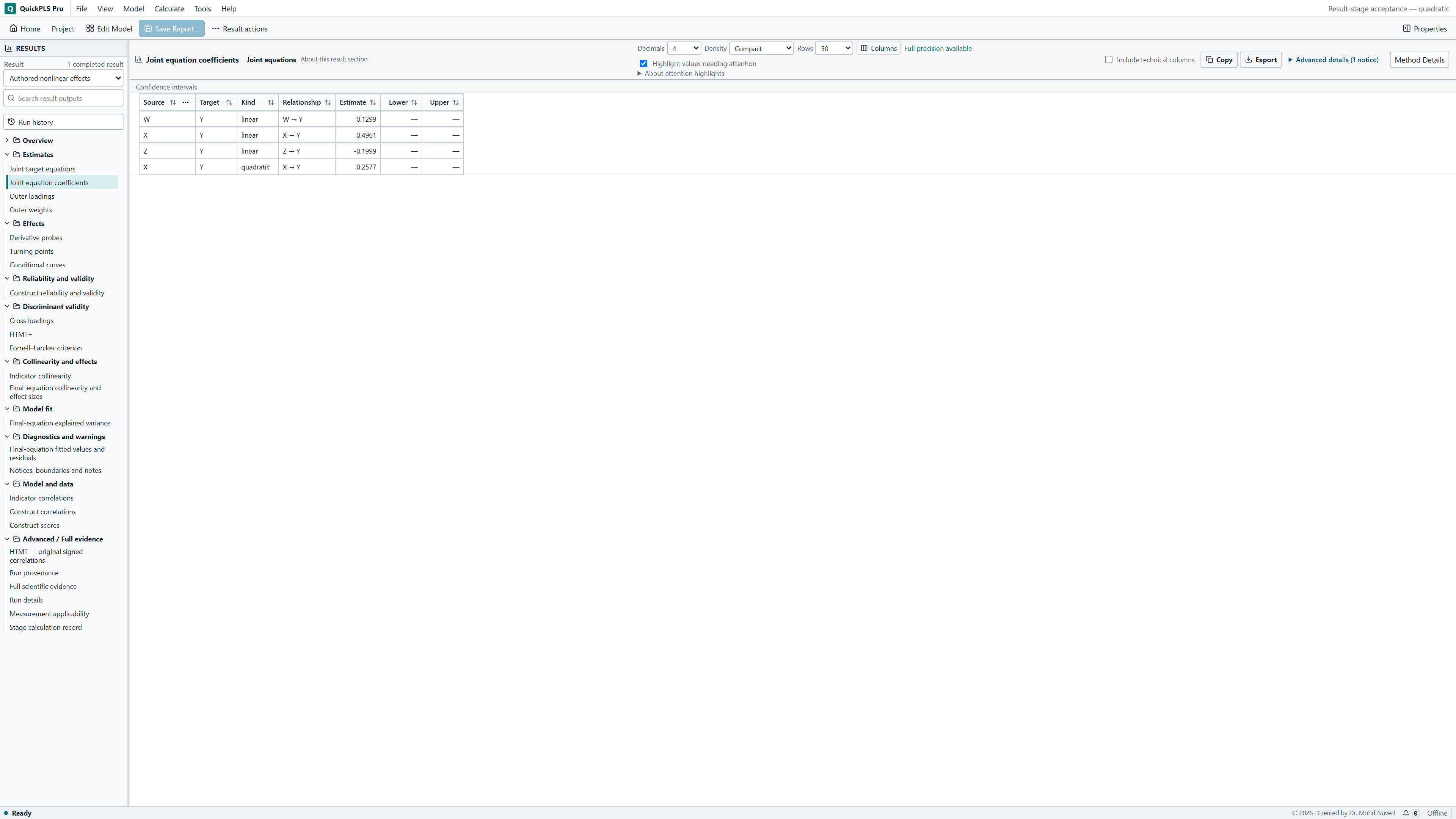
On the model, select the intended directed path. Choose Model → Quadratic Effect…. Check Predictor, Outcome and Standardized predictor², enter an Effect label, and click Add quadratic effect.
Open the nonlinear calculation
Choose Calculate… → Quadratic Nonlinear Effects. Check that the quadratic relationship you added is listed. If the workspace asks for Save and activate…, save the required project copy before starting.
Run and read the shape
Choose Point estimates, Percentile bootstrap or BCa bootstrap under Inference. Set the available bootstrap fields when needed and start the calculation. In the dedicated workspace the button is Start nonlinear analysis. Read the coefficients, curve, local slopes and inference from the same completed run.
Use the linear and square terms together
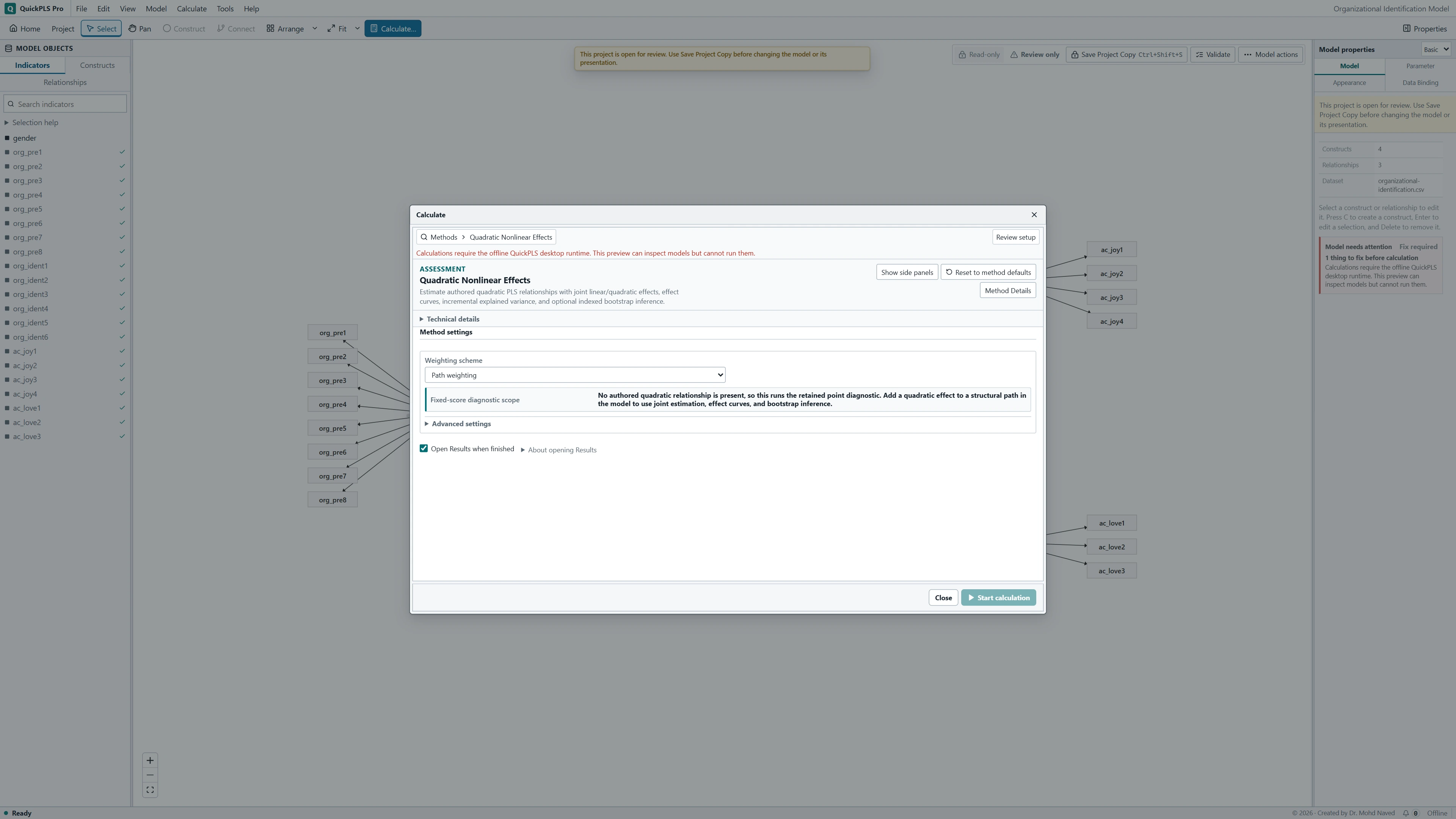
Select the completed nonlinear result. Use Search result outputs to open Joint equation coefficients, Conditional curves, Derivative probes and Turning points. Read the linear and quadratic estimates together, then inspect the local slopes and curve across the observed predictor-score range. A turning point matters only where the data support that range and contain enough cases nearby.
Check the change in R², the share of variation explained in the fitted sample, without calling it an improvement in prediction for new cases. Use intervals from the matching full-refit procedure, with its usable and failed draw counts.
On a small screen, swipe the table sideways to see every column.
| Output | How to read it | What to check |
|---|---|---|
| Linear and quadratic coefficients | The joint shape of the fitted relationship. | Neither coefficient alone describes the whole effect. |
| Effect curve / turning point | How the relationship changes over predictor values. | Extrapolated turns are not observed reversals. |
| Incremental explained variance | The increase in explained variance when the specified quadratic term is added to the fitted model. | It is not automatically better out-of-sample prediction. |
A downward bend can still be an increasing relationship
The example below uses a simple equation to show why a square coefficient and a slope are different quantities. Follow the observed range before naming the shape as a U or inverted U.
Illustrative example, not a software benchmark
For the illustrative equation y = 2x − 0.5x², the slope is 2 − x and the turning point is x = 2. If observed x values run only from 0 to 1, the observations cover an increasing segment. Calling that an observed inverted-U would overstate the evidence. These numbers illustrate the arithmetic, not QuickPLS output.
Practice: add diminishing returns to the Quality path
Use the 360-case synthetic research-workshop.csv file. Build reflective Quality, Trust, Satisfaction and Loyalty from their indicator blocks, with Quality → Satisfaction, Trust → Satisfaction and Satisfaction → Loyalty.
Retain the straight-line model as your starting specification. The planned extension adds a degree-two, or quadratic, Quality relationship to Satisfaction while keeping the original Quality path. The square is formed from the standardized predictor score, not from a separate set of squared survey items.
The arithmetic later in this guide uses hypothetical coefficients. It is a reading exercise, not an answer key showing what the CSV must produce.
Run the authored quadratic exercise
Preserve the starting model
Save the checked linear specification. Select Quality → Satisfaction on the model and choose Model → Quadratic Effect…. Confirm Quality as Predictor and Satisfaction as Outcome, then click Add quadratic effect.
What you should see: The base equation includes the focal predictor.
How to read it: Keep its linear term when adding its square.
Verify that the authored term is present
Open Calculate… → Quadratic Nonlinear Effects. The settings should list the degree-two relationship. If the screen instead says Fixed-score diagnostic scope with no authored quadratic relationship, return to the model and add the intended effect.
What you should see: The quadratic term is assigned to the intended relationship.
How to read it: Confirm predictor, outcome and scale.
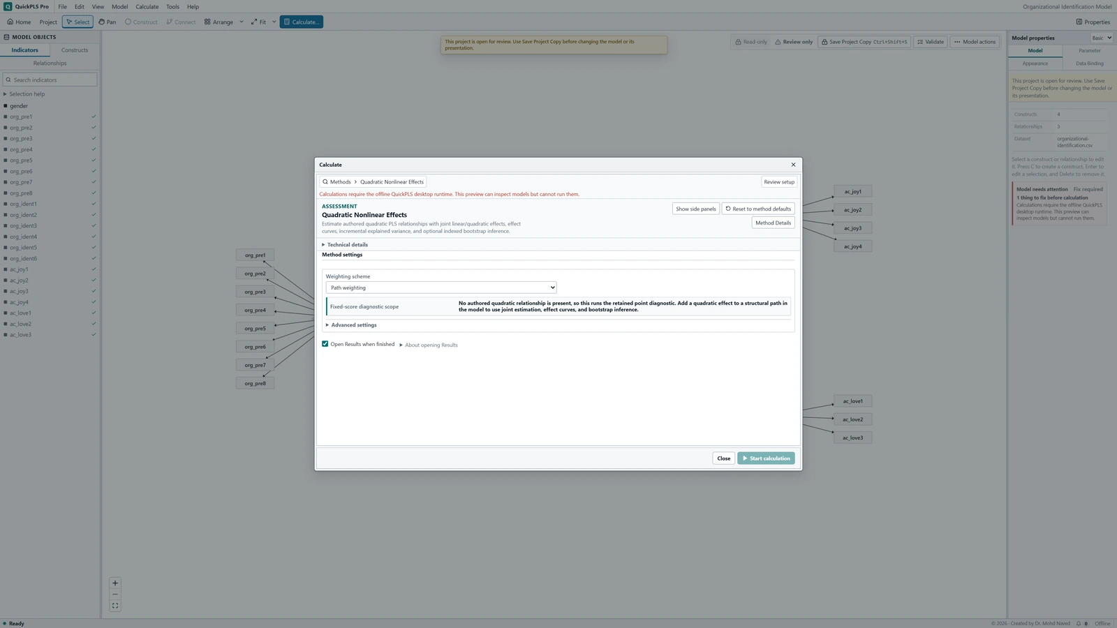
Quadratic Nonlinear Effects settings in QuickPLS. Select your own dataset and model, then use the choices described in the steps. Save and activate if requested
The nonlinear workspace can require Save and activate… to keep the original model and its results intact. Save the requested project copy and review the active model before running.
What you should see: The saved copy is active and retains the authored quadratic term.
How to read it: Check the active model before entering inference settings.
Choose the inference settings
Select Percentile bootstrap for this teaching run, with Bootstrap draws 1000, Confidence level (%) 95 and Seed 20261105. Record Workers. Point estimates and BCa bootstrap are separate choices; BCa includes additional leave-one-case-out work.
What you should see: The calculation settings and requested uncertainty are recorded.
How to read it: Resolve Readiness messages before starting.
Start and examine the completed shape
Start the calculation; the dedicated workspace labels the action Start nonlinear analysis. Read the linear and square estimates together, the 21-point curve across the observed score range, and slopes at -1, 0 and +1. Other standardized predictor scores are held at zero for this display.
What you should see: The output contains the linear and squared coefficients.
How to read it: Their combination determines the local slope.
Check the turning point and uncertainty
Compare any turning point with the observed predictor range. Inspect the matching intervals, R² change and failed-refit accounting. Do not interpret an interval from the fixed-score diagnostic as if it came from this full authored analysis.
What you should see: The curve and interval evidence support the stated interpretation over the chosen range.
How to read it: Retain the original model for comparison.
Work through the curve before naming its shape
Suppose the linear Quality coefficient is 0.30 and the square coefficient is -0.15. The slope is 0.30 + 2 × (-0.15) × Quality. At Quality values -1, 0 and +1, the slopes are 0.60, 0.30 and 0.00. The association becomes flatter as Quality rises; the negative square does not make it negative throughout the range.
The turning point is -0.30 / (2 × -0.15) = 1.00. If the observed Quality scores run from -1.8 to 1.6, that point lies within the range, although local data support still matters. If the largest observed score is 0.7, the study has not observed the predicted turn.
Suppose R² rises from 0.42 to 0.46. The increase is 0.04, or four percentage points of sample variance explained. It is not a claim of four percent better prediction for future cases. These values are hypothetical teaching numbers.
Check the model, range and influential cases
Begin with the authored relationship: a screen without that term is a different calculation. If the model is correct but the bend is uncertain, inspect the range, influential observations and inference status before drawing a shape conclusion. Use the table to choose the next check.
On a small screen, swipe the table sideways to see every column.
| Symptom | Check | Reasonable action |
|---|---|---|
| Only a fixed-score diagnostic is shown | Inspect whether the model actually contains an authored quadratic relationship. | Create and save the intended relationship, or report the narrower diagnostic. Do not claim full-refit bootstrap inference from a point-only result. |
| A turning point is absent | Check whether the squared coefficient is effectively zero or the turning point lies outside the observed range. | Describe the supported rising, falling or flattening pattern. Do not extrapolate a reversal beyond the data. |
| The linear coefficient changes sharply | Check that both linear and squared terms were fitted jointly and inspect their dependence. | Interpret the joint equation. The earlier linear-only coefficient answers a different question. |
| BCa intervals are unavailable | Read failed resamples and leave-one-out failures. | Report the unavailable BCa result. If a separately justified percentile analysis is used, identify that change rather than silently substituting it. |
| A curve looks precise near the centre but uncertain at the ends | Inspect sparse observations and interval width across the observed range. | Limit interpretation at poorly supported extremes. Do not crop the plot to conceal uncertainty. |
Check whether the bend survives reasonable scrutiny
Compare the planned linear and quadratic specifications using the same intended variables and cases. Inspect the fitted curve and uncertainty rather than treating a threshold crossing as the only useful result. Examine unusually influential cases, but do not delete them solely to make curvature significant.
The full bootstrap rebuilds the relevant scores and squared term in each resample. The inference procedure requires at least 90% usable fits; BCa also uses leave-one-case-out calculations. Investigate failures or unavailable intervals rather than replacing them with zero or silently dropping them.
If a turning point is poorly supported, report diminishing or increasing slopes over the observed range instead of claiming an optimum. Treat unplanned transformations or extra curves as exploratory and assess prediction separately if future performance is the objective.
Describe the observed bend in ordinary language
Methods example: We retained the linear Quality → Satisfaction path and added an authored quadratic Quality effect. We fitted the two terms together, examined the curve over the observed standardized score range and used the stated full-refit bootstrap for uncertainty. Add the actual settings and retained-case count.
Results example: The hypothetical linear and square coefficients were 0.30 and -0.15. The local slope fell from 0.60 at Quality = -1 to zero at +1, with a turning point at 1.00. We interpreted that point only after checking observed support. R² increased by 0.04; this described sample fit rather than validated prediction. Replace all hypothetical values with your completed result.
| Field | Report |
|---|---|
| Specification | The quadratic relationships added to the model and their matching linear relationships. |
| Scale | Standardisation, observed range and other scores held fixed. |
| Estimates | Joint coefficients, local slopes, turning-point status and incremental R-square. |
| Inference | Interval method, confidence, attempted/usable/failed draws and seed. |
| Interpretation | Supported curve shape, uncertainty and limits on extrapolation. |
Can you explain what the curve actually shows?
- Confirm that the saved model contains the intended quadratic effect and its linear parent path.
- Explain why the square coefficient is not the slope at every predictor value.
- Read the local slopes and check the turning point against the observed range.
- Distinguish an authored full-refit analysis from a fixed-score diagnostic.
- Report uncertain curvature or an unsupported turning point honestly instead of forcing a U-shaped conclusion.
Report the shape and where it was observed
- State why curvature was expected and identify the retained linear path and authored square.
- Report the score scale, linear and square coefficients, local slopes and any turning point within the observed range.
- Give the R² comparison and distinguish sample fit from prediction on new cases.
- Describe the inference procedure, refitted quantities, bootstrap settings and failures.
Keep the curve within what the data can show
A square tests one particular form of curvature, not every possible nonlinear shape. A quadratic equation continues beyond the data, but the study does not automatically support that extension. A calculated turning point beyond the observed score range is not an observed optimum.
Curvature can also reflect a few influential cases, an omitted relationship or measurement problems. Examine these explanations before using the curve as a practical recommendation. Adding flexibility is not, by itself, evidence of a better research model.