 QuickPLS
What the method does
Prospective simulation estimates how often a planned test detects an effect when data are generated under a declared population model. The result depends on the assumed path, indicator loadings, test and candidate sample sizes. QuickPLS’s planning workflow uses a two-construct reflective model with one path; these assumptions should match the planning question.
Estimated power at n = number of planned simulations rejecting the null / number of planned simulations.
Each candidate sample size has a simulation estimate and an interval describing Monte Carlo uncertainty. QuickPLS’s conservative choice uses the interval’s lower bound against the target. Failed planned replicates remain relevant to the denominator; additional simulations reduce Monte Carlo uncertainty rather than uncertainty about the population assumptions.
Data and analysis in QuickPLS
Specify two reflective constructs, one population path, the indicator loadings, candidate sample sizes and simulation settings. This planning calculation uses declared assumptions rather than treating an observed dataset as the population.
QuickPLS runs the simulation plan and reports power by sample size. Examine alternative plausible effects and loadings before choosing a recruitment target.
Follow a worked example
The following example shows the data, settings and decisions for one analysis. Use the linked practice files to follow it. For your own study, keep the procedure and choose the variables, model and settings that fit your research question.
This example plans a Quality to Satisfaction study from assumed loadings and a population path. You do not need to collect observations first. The optional research-workshop.csv file has 360 rows and 31 columns and can help you create the named model; the power calculation generates its own data from the assumptions you enter.
How many cases should you plan for a simple PLS study?
Before collecting data, choose the smallest relationship your study needs to detect and reasonable assumptions about measurement quality. PLS-SEM Sample Size and Power repeatedly generates data under those assumptions and fits the planned model. Estimated power is the proportion of planned simulations in which the test detects the assumed relationship.
This guide covers two reflective constructs connected by one path. You compare a list of possible sample sizes and see which evaluated size meets the target conservatively. The result depends on the assumed effect and loadings, so the useful starting point is a defensible scenario rather than a desired sample-size answer.
Practice: plan a Quality → Satisfaction study
Use a separate model with only Quality and Satisfaction, each measured by three reflective indicators, and Quality → Satisfaction as its only path. The workshop file can help you create and name those indicator blocks.
The calculation generates new data from the scenario you enter. It does not resample the 360 uploaded workshop rows as its population. Treat the chosen path and loadings as explicit planning assumptions.
Use the short teaching run below to learn the fields and outputs. A real research plan should justify its effect and loading assumptions and use enough simulation repetitions for a stable decision.
Prepare a simple model and defend the assumptions
Use exactly two ordinary reflective constructs, each with 3 to 10 indicators, and one directed path. Reflective means that each construct explains its indicator responses. You will supply the assumed population path and an expected loading, the strength of its measurement relationship, for every indicator; these are planning assumptions, not estimates automatically borrowed from the uploaded data.
The simulation generates normally distributed latent variables and independent errors under its supported design. It does not reproduce an entire complex study with groups, weights, missingness, interactions or clustered observations. Choose a different planning approach when those features are central to your study.
Enter a scenario and compare sample sizes
Choose the planning method
Open Calculate… → PLS-SEM Sample Size and Power for the two-construct model. Enter a Scenario identity and choose Predictor construct and Outcome construct.
Enter the assumptions
Set Predictor loadings and Outcome loadings in the displayed indicator order, Population path and Sample-size grid. Then set Two-sided alpha, Target power and Wilson confidence level. The Wilson field uses a percentage.
Set the simulation and inspect the result
Enter Monte Carlo replicates per grid point, Case-bootstrap replicates per dataset and Parallel workers. Record the seed in Advanced settings and review Pre-run desktop workload. Start calculation, then read Power by sample size and the conservative grid decision.
Enter the teaching scenario carefully
Choose the two constructs
Create and save a separate model containing only Quality from quality_1, quality_2 and quality_3 and Satisfaction from satisfaction_1, satisfaction_2 and satisfaction_3, both Reflective, with Quality → Satisfaction as its only path. Open Calculate… → PLS-SEM Sample Size and Power. Enter a clear Scenario identity and choose Quality as Predictor construct and Satisfaction as Outcome construct. Verify the displayed indicator order.
What you should see: The design contains exactly the supported two reflective constructs and one path.
How to read it: Use a different planning approach for another design.
Enter the population assumptions
Set Population path to 0.20 and every Predictor loading and Outcome loading to 0.80. The path is an assumed population relationship, not a requested result. The supported path range is -0.80 to 0.80 and each loading must be between 0.50 and 0.95.
What you should see: Population path and indicator loadings are entered as assumptions.
How to read it: They are not estimates from the future study.
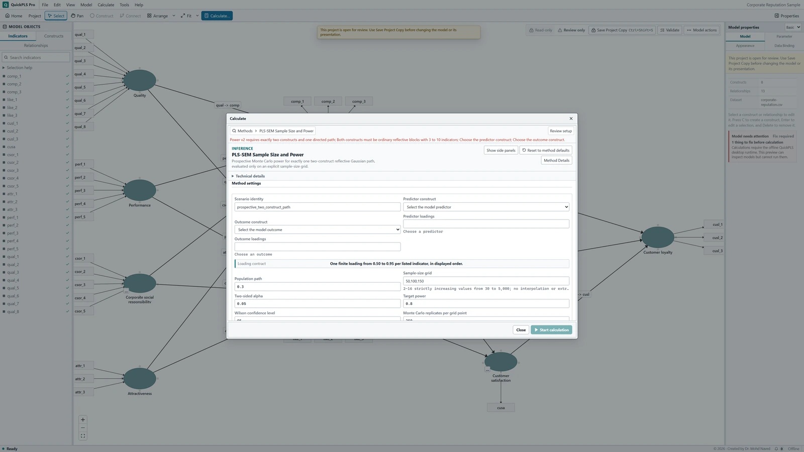
PLS-SEM Sample Size and Power settings in QuickPLS. Select your own dataset and model, then use the choices described in the steps. Enter the evaluated sample sizes
Set Sample-size grid to 100, 200, 300. It must contain 2 to 16 strictly increasing sizes from 30 to 5000. The calculation evaluates those rows; it does not fill the gaps automatically.
What you should see: The candidate sizes are ordered and valid.
How to read it: The calculation evaluates those sizes rather than every possible sample size.
Set the decision rule
Enter Two-sided alpha 0.05, Target power 0.80 and Wilson confidence level 95. This field is a percentage: 95 corresponds to the proportion 0.95. Do not enter 0.95 into the percentage field.
What you should see: Alpha, target power and interval level define the decision.
How to read it: Record them before examining the power curve.
Set the teaching run size
Use Monte Carlo replicates per grid point 100 and Case-bootstrap replicates per dataset 99. Record Seed 20261105 and the chosen Parallel workers. The supported outer count is 100 to 10000; the inner count must be an odd number from 99 to 1999. Review Pre-run desktop workload before starting. Monte Carlo replicates are the newly generated datasets; the case-bootstrap replicates are resampled fits within each dataset.
What you should see: Simulation and bootstrap counts, seed and workers are recorded.
How to read it: More replicates address simulation uncertainty, not incorrect population assumptions.
Choose from the completed rows
Start calculation and open Power by sample size. Find the first evaluated row whose lower Wilson bound reaches 0.80. If no row meets that rule, report that the evaluated grid did not reach the target; review assumptions or extend the grid for a separately saved scenario.
What you should see: Each candidate row shows power and its interval.
How to read it: Choose only under the stated lower-bound rule; retain a result that reaches no target.

Use the lower confidence bound to select an evaluated size
Open Power by sample size. Each row describes one size you actually evaluated, its estimated power and its Wilson interval. A Wilson interval shows uncertainty caused by running a finite number of simulations. The conservative decision uses the first row whose lower bound reaches your target.
Also inspect Bootstrap tail accounting and Simulation failures. Failed outer simulations remain in the planned denominator, so removing them from your own arithmetic would make the result more optimistic. The Power curve helps compare rows, but it does not establish an exact minimum between them.
On a small screen, swipe the table sideways to see every column.
| Output | How to read it | What to check |
|---|---|---|
| Design assumptions | Population path, measurement loadings and distribution used in simulation. | They should represent a plausible planned study. |
| Power at each tested N | The simulated detection proportion for that grid point. | The calculation does not establish power at sample sizes between those tested. |
| Simulation uncertainty / failures | How precisely power was estimated and whether simulated analyses could be completed. | A rounded proportion alone hides simulation variability. |

Why estimated power above the target may not be enough
Suppose the target is 80% power. At sample sizes 100, 200 and 300, hypothetical power estimates are 0.60, 0.82 and 0.90. Their lower 95% Wilson bounds are 0.50, 0.73 and 0.83. The 200-case point estimate exceeds 0.80, but its lower bound does not. The first qualifying evaluated size is 300.
This does not prove that 300 is the exact minimum or that every size between 200 and 300 fails. If that range matters to the decision, evaluate a more informative grid in another documented scenario rather than interpolating a guaranteed answer.
Suppose 80 detections occur in 100 planned simulations, of which 90 produce usable completed analyses. The planned-denominator estimate is 80 / 100 = 0.80. It is not 80 / 90. Failed outer simulations remain in the denominator, and an individual dataset needs at least 90% usable inner bootstrap fits for its test.
The teaching workload has 3 × 100 × 99 = 29,700 inner bootstrap fits, in addition to the original dataset fits. This explains why even a small grid can take noticeable time. It is a fit count, not a promised running time.
A qualifying grid point is not an exact population minimum
The result identifies a size on the list you supplied under the stated model and simulation assumptions. The example below explains why a neighboring unevaluated size cannot be declared sufficient or insufficient from that decision alone.
Illustrative example, not a software benchmark
Suppose 250 is the smallest tested sample size meeting your criterion. The finding concerns 250 under the simulated design. It does not prove that 249 is inadequate or that 250 is enough for a different model. Explore plausible weaker paths and less reliable measurement before deciding on recruitment.
When the target is not reached or results are unstable
Check whether the issue is a blocked setup, simulation failure or a valid result below target. These require different responses. Fix an unsupported model or invalid input first; for a completed run, review the failure counts, uncertainty and scenario assumptions before changing the grid.
On a small screen, swipe the table sideways to see every column.
| Symptom | Check | Reasonable action |
|---|---|---|
| The model is ineligible | Exactly two reflective constructs, one path and three to ten indicators per block | Use the stated profile for this exercise. A complex study needs a power method that represents its actual design. |
| Target not reached | Largest evaluated size and lower Wilson bounds | Extend a justified grid or reconsider feasibility. Do not inflate the assumed effect simply to obtain a smaller number. |
| Estimated power is not perfectly increasing | Simulation uncertainty and replicate count | Inspect intervals and increase a declared simulation budget if needed; do not manually smooth results. |
| Many simulated datasets fail | Convergence, ordinary PLS settings without a consistency correction, and usable inner-bootstrap counts | Diagnose failures and retain them in the planned denominator rather than deleting them. |
| A pilot implies exceptionally high power | Whether the effect and loadings were optimistically selected | Evaluate plausible weaker effects and measurement quality before committing to recruitment. |
Plan for plausible weaker effects and measurements
Repeat the plan under assumptions that would matter in practice. For example, compare a population path of 0.15 with 0.20, and indicator loadings of 0.70 with 0.80. Explain why those scenarios are plausible for the planned study.
The current simulation uses a null-centered, two-sided bootstrap test with an added-one correction to its tail probability. Failed fits are counted and are not silently retried until a success appears. Read those counts when comparing scenarios.
Increase simulation repetitions when Monte Carlo uncertainty prevents a clear decision. Keep the same declared scenario when assessing simulation stability; changing the effect, loadings and grid at the same time makes the source of any changed recommendation hard to understand.
Separately consider recruitment losses and study features such as subgroups or nonnormal measurements. Do not claim the simple normal-data scenario already covers them.
Report the scenario so someone else can repeat it
- Specify the two reflective constructs, indicator counts, population path and ordered loadings.
- Report the sample-size grid, alpha, target power, Wilson confidence level, simulation counts, seed and workers.
- Give power estimates and intervals, failed simulations and the first evaluated size meeting the lower-bound rule.
- Explain the design assumptions and any further allowance needed for attrition, missingness or study features outside this simulation.
Write the planning assumptions and conservative decision
Methods example: We simulated a two-construct reflective model with population path 0.20 and indicator loadings 0.80. We evaluated sample sizes 100, 200 and 300 using two-sided alpha 0.05, target power 0.80 and 95% Wilson intervals. The decision rule selected the first evaluated size whose lower interval bound met the target. Add the actual repetition counts, seed, workers and failure accounting.
Results example: In the hypothetical illustration, estimated power at 200 cases was 0.82 with lower bound 0.73. At 300 cases it was 0.90 with lower bound 0.83, so 300 was the first qualifying grid point. This was a recommendation under the stated assumptions, not proof of an exact minimum. Replace these example values with the saved simulation results.
| Report item | Detail to retain |
|---|---|
| Population model | Path, loadings, distributions and independence assumptions |
| Grid | Every evaluated sample size |
| Decision | Alpha, target power and Wilson confidence level |
| Simulation | Planned replicates, inner bootstrap count, seed and failures |
| Conclusion | First qualifying evaluated size or target not reached; sensitivity scenarios |
Check the recommendation before using it for recruitment
- Explain and justify the population effect and every loading assumption.
- Confirm that the planned study fits the supported two-construct, one-path design.
- Show why an estimated power of 0.82 does not by itself satisfy a conservative target of 0.80.
- Use the planned denominator and report simulation failures.
- Name the first qualifying evaluated size and distinguish it from an exact minimum or a post-hoc adequacy claim.
Match the planning model to the future study
This is prospective simulation for the declared simple design. It is different from the post-hoc study-wide minimum and historical per-path technical-power projections based on fitted coefficients.
A supported simulation can still be a poor plan if the assumed effect is too large or the indicators are stronger than those you will use. More simulation repetitions reduce simulation uncertainty; they do not repair unrealistic assumptions.
Saved historical results retain their original method identity. The earlier prospective procedure failed its calibration check and was replaced by a different inference procedure. Do not relabel an earlier result as the current calculation or mix their probabilities in one planning conclusion.