 QuickPLS
What the method does
NCA looks for an empty upper-left region in a condition-outcome plot: high outcomes that do not occur when the condition is low. A ceiling line describes that constraint. Effect size summarises the empty region, and a bottleneck table translates outcome targets into minimum-condition levels under the selected ceiling.
Necessity effect size: d = C / S.
C is the area of the ceiling zone and S the scope of the analysed plot. Both depend on the chosen ceiling and bounds. A necessary condition can still be insufficient: meeting the minimum does not guarantee the outcome.
Data and analysis in QuickPLS
Use numeric condition and outcome observations in rows. Examine their ranges, outliers, missingness and whether the direction of the proposed necessity makes sense.
QuickPLS calculates the ceilings, effect sizes and bottleneck tables. Inspect the plot and the units of each threshold before applying the result to your research question.
Follow a worked example
The following example shows the data, settings and decisions for one analysis. Use the linked practice files to follow it. For your own study, keep the procedure and choose the variables, model and settings that fit your research question.
Download research-workshop.csv to begin. It contains 360 rows and 31 columns. The example below identifies the variables to use, their roles and any rows to exclude; not every column is an analysis variable.
Study question: what does high performance require?
Does high innovation performance require a minimum level of digital capability? The first exercise examines this question using 180 synthetic cases. A subsequent workshop compares Quality and Trust as possible requirements for Satisfaction on a separate dataset.
Necessary condition analysis (NCA) examines the empty region towards the upper left of a condition-outcome plot, with the condition on the horizontal axis and the outcome on the vertical axis. This region represents combinations of a high outcome and a low condition that do not occur in the analysed sample.
A ceiling describes the boundary of that region. Its effect size is the empty area relative to the selected analysis range. Bottlenecks translate the ceiling into minimum condition levels for specified outcome targets. Cases below a requirement cannot reach the target under the fitted ceiling; cases above it may still fall short.
Data and analysis plan for the checked exercise
Download innovation-necessity.csv and its data notes. The file contains 180 invented cases, with digital_capability as the condition and innovation_performance as the outcome. Keep the original units and use all 180 complete cases.
Confirm that larger values indicate more capability and performance. Inspect missing values, impossible entries, observed minima and maxima, and unusual cases near the boundary. Use the observed ranges for this baseline.
The later Quality-and-Trust workshop uses different variables and data. Its instructions extend the method; the checked numerical answers for innovation-necessity.csv are not answers for that workshop.
Run the digital-capability analysis
CE-FDH constructs a stepped ceiling. CR-FDH fits a line from the observations defining the boundary. Their geometry differs, so comparing both assesses the same proposed requirement under two ceiling constructions.
Permutation analysis rearranges the observed values and recalculates the statistic for comparison. The seed makes the random sequence repeatable under the same setup. The independent answer check covers ceilings and bottlenecks; it does not establish matching permutation probabilities across packages.
Before starting, check the variable names, Permutations and Seed against the steps above. After the calculation finishes, select its result and confirm that all 180 cases were analysed. Keep this result separate from the optional two-condition workshop.
Open the single-condition setup
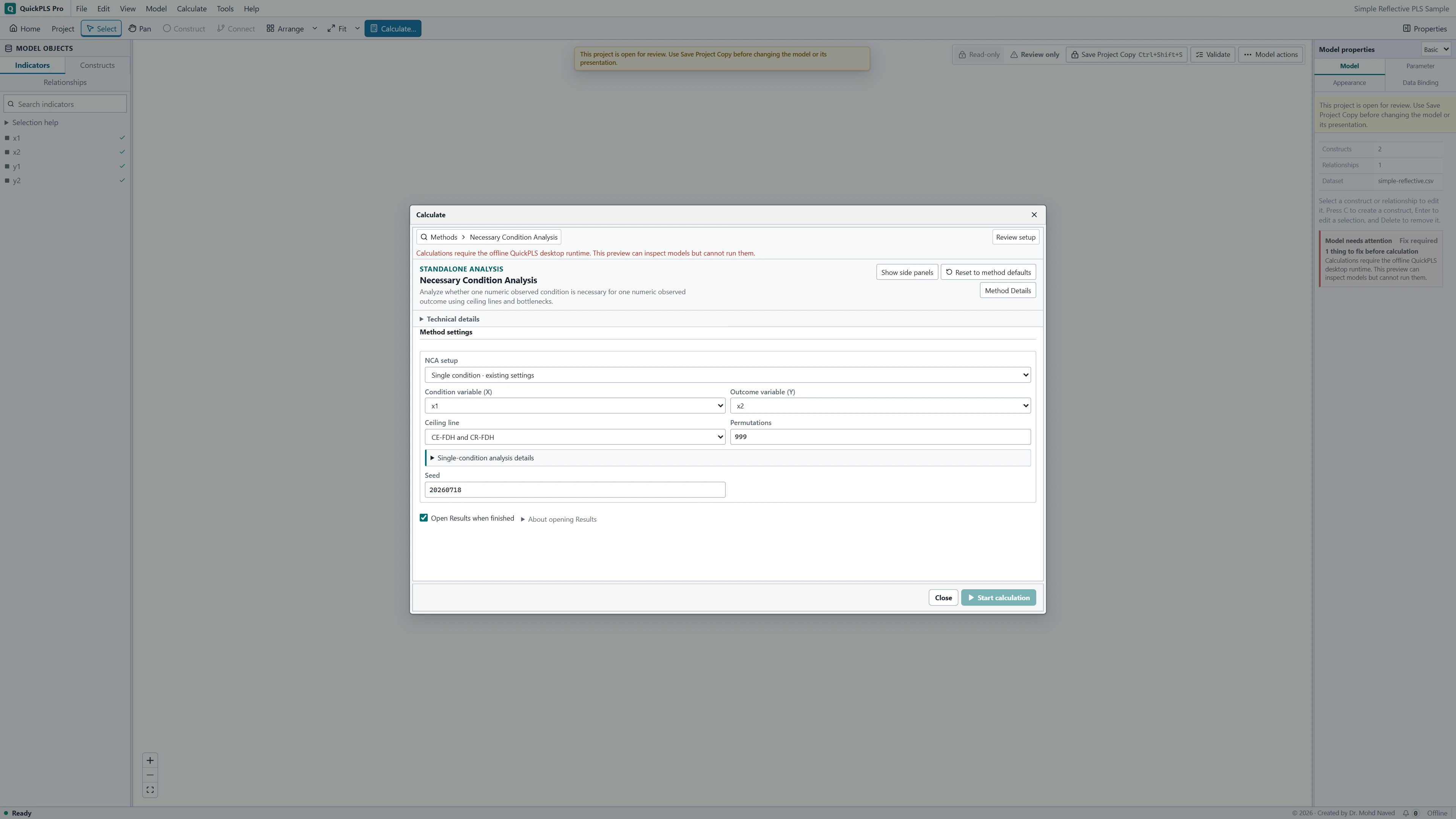
Import innovation-necessity.csv into the intended project. Open Calculate → Necessary Condition Analysis and select Single condition · existing settings under NCA setup.
What you should see: The NCA settings show the single-condition variable selectors for innovation-necessity.csv.
Assign the variables and ceilings
Set Condition variable (X) to digital_capability and Outcome variable (Y) to innovation_performance. Set Ceiling line to CE-FDH and CR-FDH. The checked analysis uses original units, observed ranges and listwise deletion, which keeps rows complete on the required variables. All 180 cases in this file are complete. These describe the single-condition calculation; they are not additional selectors in this setup.
What you should see: The two variable roles and both ceiling methods are selected.
Set the permutation plan and calculate
Use 999 permutations and Seed 20261106 for the checked setup. Start calculation, select the completed result and confirm its case count and variable roles before comparing the answers below.
Checked ceiling and bottleneck results
Begin with the ceiling and the observations defining it. The effect size quantifies the empty area relative to the chosen range rectangle. The bottleneck table expresses the minimum condition level implied for each outcome target. Read the ceiling method, target and units together.
For innovation-necessity.csv, the checked CE-FDH effect size is 0.406223 and the CR-FDH effect size is 0.386317. The CR-FDH slope is 0.996655 and its intercept is 8.525243. These coefficients describe the fitted ceiling, not an average regression relationship.
At 80% of the observed performance range, the capability requirement is 72.1364% of the observed capability range under CE-FDH and 68.3858% under CR-FDH. An outcome at 80% of its observed range is not automatically a raw score of 80.
These practice results were calculated by running the QuickPLS calculation code outside the desktop app. All 88 numerical and status checks agreed with NCA 5.0.2 under the recorded comparison rules. The check covers ceilings and bottlenecks; permutation probabilities were not independently matched.
In Results, open Ceiling effect sizes and permutation inference for the two effect sizes, CR-FDH ceiling coefficients for the line, and Observed-range bottlenecks for the target-specific requirements. CE-FDH frontier peers identifies the observations defining the stepped ceiling. Compare the same ceiling method and target with the answers below.
On a small screen, swipe the table sideways to see every column.
| Output | How to read it | What to check |
|---|---|---|
| CE-FDH / CR-FDH ceiling | Two supported ways to describe the boundary of the attainable observations. | Their geometry and results need not be identical. |
| Effect size and permutation probability | The relative empty space and its configured inferential assessment. | A small probability does not identify a causal mechanism. |
| Bottleneck table | The minimum condition level implied by the ceiling for each outcome target within the selected range. | Distinguish no requirement, unavailable and unattainable results. |

Interpret a bottleneck as a necessary, not sufficient, level
Interpretation of a minimum requirement
Under the selected ceiling and analysis range, an outcome target is not supported below the reported condition requirement. Cases above that requirement can still fall short of the target. Digital capability may therefore be necessary for high performance while other resources or circumstances remain insufficient.
Troubleshooting and analytical diagnosis
Verify the variable roles, coding direction, case count and analysis ranges before interpreting an unexpected result. Reversing the outcome or changing the rows changes the question being analysed.
For the 180-case answer check, use the exact innovation-necessity.csv file with both planned ceilings and observed ranges. Resolve setup differences before assessing agreement with the reference values.
When the setup is correct, a small effect or uncertain permutation result may be the substantive finding. The checks below distinguish input errors, geometric differences between ceilings and limits to the evidence.
On a small screen, swipe the table sideways to see every column.
| Symptom | Check | Reasonable action |
|---|---|---|
| One observation changes the ceiling sharply | Data accuracy and frontier-defining cases | Correct actual errors; report a justified sensitivity analysis for valid unusual cases. |
| CE-FDH and CR-FDH disagree | Ceiling geometry and point placement | Explain the difference and report both if both were planned. |
| A theoretical range is rejected | Whether all included values lie within the bounds | Correct or justify the bounds; do not discard inconvenient cases to fit them. |
| A bottleneck entry is unavailable | Target, range and ceiling status | Report the status rather than converting it to zero. |
| Condition comparisons use different cases | Shared complete-case requirements | Use the common-sample setup for the planned comparison. |
| ESSE is described as deleting 5% of cases | The joint-distribution threshold and unchanged range | Describe the actual threshold analysis and its sequence. |
Methods and results examples
For the checked 180-case capability example, CE-FDH and CR-FDH effect sizes are 0.406223 and 0.386317. Report the ceiling, range and target with each bottleneck requirement. Identify these as synthetic practice results calculated by QuickPLS code outside the desktop app; the independent comparison covers ceilings and bottlenecks, not permutation probabilities.
In an empirical report, replace the examples with the saved calculation's sample, settings, effect sizes, probabilities and requirements. Explain unavailable requirements and any sensitivity that materially changes the interpretation.
| Item | Report |
|---|---|
| Variables | Condition and outcome definitions, direction and score origin |
| Cases and ranges | Common sample, exclusions and bounds |
| Ceiling | CE-FDH, CR-FDH or both |
| Effect and inference | Effect size, permutation count, seed and probability convention |
| Bottlenecks | Target grid, units, requirements and unavailable statuses |
| Sensitivity | Threshold sequence, fixed range and effect changes |
Reporting the optional workshop and arithmetic illustration
Methods example for the workshop: We examined quality_mean and trust_mean as possible necessary conditions for satisfaction_mean using the same complete cases. We used empirical ranges and compared CE-FDH with CR-FDH. We recorded the permutation settings and expressed bottlenecks in original units and percentages of the declared ranges. CE-FDH sensitivity was assessed at prespecified joint-distribution thresholds with the ranges held fixed.
Results example for the hypothetical arithmetic: An empty ceiling area of 20 within a range area of 100 gave an effect size of 0.20. The illustrative 80% outcome target required 35% of the condition range. This was a minimum boundary requirement rather than a guarantee of attaining the target. These values demonstrate interpretation; they were not calculated from the workshop CSV.
Essential information for an NCA report
- Define the condition and outcome, coding direction, score origin, analysis bounds and ceiling method.
- State the analysed sample and any exclusions. Identify influential frontier observations and explain documented corrections or sensitivity analyses.
- Report the effect size and permutation procedure, count and seed. For each bottleneck, specify the outcome target, condition requirement, units and status.
What the analysis establishes
NCA characterises a minimum requirement under a ceiling and range. Regression characterises an average relationship. Evidence for either does not substitute for the other.
A causal interpretation requires a substantive argument about the measures, sampling and design in addition to the observed boundary. Retain any status indicating that a requirement could not be calculated, and explain how it limits the conclusion.
Exercises and final analysis record
- Identify the original observations defining each ceiling and explain any difference between CE-FDH and CR-FDH.
- Convert a reported requirement from a percentage of the declared range to original units.
- Explain why meeting a minimum requirement does not ensure the outcome.
- Distinguish no requirement from unavailable and unattainable results.
- Verify that Quality and Trust were analysed on the same complete cases.
- Explain how an ESSE threshold comparison differs from deleting cases and shrinking the empirical range.
Optional methods and settings
Workshop: Quality and Trust as requirements for Satisfaction
Use research-workshop.csv for this extension. The question is whether high Satisfaction is absent below a minimum level of Quality or Trust. Compare both conditions on the same rows.
Select quality_mean and trust_mean as conditions and satisfaction_mean as the outcome. These supplied columns are arithmetic means of the named indicators, not latent-variable estimates or fitted PLS scores.
Read the data guide, confirm the ranges and inspect unusual observations. Larger values indicate more of the named condition or outcome. The synthetic labels provide a context for learning the procedure rather than evidence of an empirical necessity relationship.
This workshop has no checked numerical answers on this page. Use the earlier 180-case capability exercise when you need an exact result comparison.
Extend the analysis to several conditions
The configurable setup compares several proposed requirements for one outcome. Use a shared complete-case sample containing values for every selected condition and the outcome. Otherwise, a difference between conditions may reflect different analysed cases.
Empirical bounds use observed minima and maxima. Theoretical bounds use limits justified by the measurement scale or research question. They must contain every included value. Widening the bounds changes the range rectangle used to calculate effect size and may change the meaning of an outcome percentage.
Choose the target levels and requirement units before comparing the conditions. An original-unit requirement and a percentage of the declared range express the same boundary in different units only when the bounds are known.
Choose the configurable analysis
Set NCA setup to Multiple conditions and configurable bottlenecks. Assign Outcome variable (Y) and Condition variables (X) from the same numeric dataset.
Specify ceilings and ranges
Set Ceiling line to CE-FDH, CR-FDH or both. Record Permutations and the seed. Under Analysis ranges select empirical bounds or justified theoretical bounds containing every included observation.
Specify the bottleneck display
Set Outcome levels, Bottleneck levels and Default requirement view. Identify whether requirements will be interpreted in original units or percentages of the declared ranges.
Choose a sensitivity analysis if planned
Enable Include CE-FDH sensitivity analysis (ESSE) to examine the boundary under Joint-distribution thresholds from 0 to less than 1. Keep the baseline range fixed and read each condition and ceiling separately after calculation.
Calculate the two-condition workshop
Open the configurable setup
With research-workshop.csv selected, open Calculate → Necessary Condition Analysis. Set NCA setup to Multiple conditions and configurable bottlenecks. Single condition · existing settings is the separate simpler route.
What you should see: The configurable multiple-condition setup is open.
How to read it: It is distinct from the simpler single-condition route.
Assign the outcome and conditions
Set Outcome variable (Y) to satisfaction_mean and Condition variables (X) to quality_mean and trust_mean. Confirm their coding direction and the shared complete-case count.
What you should see: Y is satisfaction_mean; X contains quality_mean and trust_mean.
How to read it: Check that high values have the intended meaning.
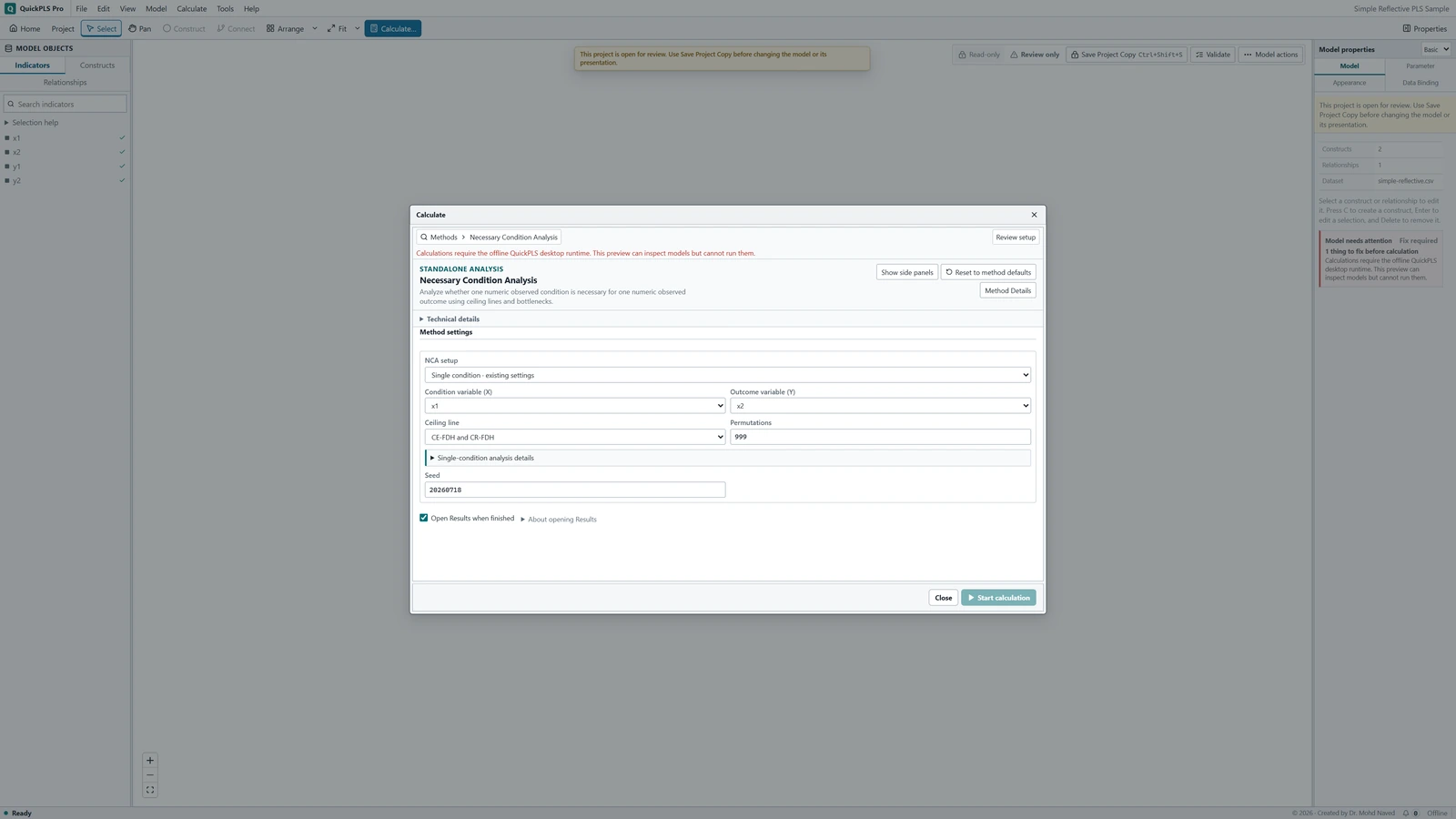
Necessary Condition Analysis settings in QuickPLS. Select your own dataset and model, then use the choices described in the steps. Select the ceiling comparison
Set Ceiling line to both CE-FDH and CR-FDH. Record Permutations and Seed. The two constructions need not return the same effect or requirement.
What you should see: Both CE-FDH and CR-FDH are selected.
How to read it: Differences between their results reflect different ceiling constructions.
Use empirical bounds for the baseline
Under Analysis ranges select empirical bounds. A later calculation with justified theoretical bounds should be saved as a separate comparison, with every included value inside the bounds.
What you should see: Empirical bounds are selected for the baseline.
How to read it: The area and effect size depend on those bounds.
Choose outcome targets and units
Set Outcome levels, Bottleneck levels and Default requirement view. Use a short sequence of meaningful targets and record whether the requirements are original-unit values or percentages of the declared ranges.
What you should see: Outcome targets and requirement units are explicit.
How to read it: A percentage requirement is not automatically an original-unit threshold.
Calculate the planned sensitivity sequence
Under Effect-size sensitivity enable Include CE-FDH sensitivity analysis (ESSE). For the sensitivity exercise below, enter Joint-distribution thresholds 0, 0.01 and 0.05. Start calculation, open the completed result and confirm its variables, common sample and ranges. Read baseline ceilings, bottlenecks and threshold results as separate outputs.
What you should see: The result contains the two-condition baseline and requested sensitivity sequence.
How to read it: Read each ceiling, bottleneck and threshold result under its own definition.
Inspect the frontier and effect size
The observations defining the upper-left boundary determine the ceiling. Inspect their original values, particularly when an unusual case has a large influence. Correct an entry only when its error is established; a valid unusual observation is part of the evidence.
CE-FDH follows a stepped boundary, whereas CR-FDH fits a regression-based ceiling from boundary observations. Uneven spacing and influential frontier cases can affect them differently. Investigate the geometry when their results diverge.
For an arithmetic illustration, an empty ceiling area of 20 within a range rectangle of 100 gives 20 / 100 = 0.20. This is an area proportion, not an R-square of 0.20 or a claim about 20% of participants.
Read a permutation probability with its procedure, count and seed. It concerns the specified comparison, while measurement error, restricted ranges and sampling can also explain aspects of the observed boundary.
On a small screen, swipe the table sideways to see every column.
| Output | Hypothetical example or check | Reading |
|---|---|---|
| Ceiling plot | Identify observations defining the upper-left boundary | Check unusual cases and direction before interpreting necessity. |
| Effect size | Empty area 20 / range area 100 = 0.20 | Relative empty space under the selected range and ceiling. |
| Permutation result | Record actual probability, count and seed | Evidence from the specified permutation test; it does not establish causation. |
| Bottleneck requirement | Hypothetical target 80% requires condition 35% | Percentages refer to the declared ranges, not participant proportions. |
| Below-requirement count | Cases strictly below the stated requirement | A count of cases is distinct from the effect-size area. |
| Status | No requirement, unavailable or unattainable | These labels cannot all be represented by zero. |
Convert a bottleneck to the original measurement units
Suppose a hypothetical bottleneck table reports that an outcome target of 80% requires a condition level of 35%. Identify both declared ranges before interpreting the entry. The fitted ceiling does not support the target below the requirement, although cases above it may still miss the target.
With condition bounds of 10 and 30, the range width is 20. The requirement is 10 + 0.35 × 20 = 17 in original units. The reported 35% is a position within that range, rather than 35% of the condition mean or 35% of participants.
Compare several conditions at the same outcome targets and on the shared sample. A comparison based on different rows mixes condition differences with sample differences.
Interpret status labels separately. No requirement, called not necessary in the checked answer pack, means that the ceiling imposes no condition requirement at the target. Unavailable means that a requirement could not be provided. Unattainable means that the target cannot be reached under the stated ceiling and range. Replacing these labels with zero changes their meaning.
ESSE: sensitivity to the CE-FDH boundary rule
ESSE examines how the CE-FDH effect changes under a sequence of boundary rules. The analysis helps establish whether a proposed requirement depends strongly on a small part of the observed frontier.
At a candidate boundary point, the relevant proportion is P(X ≤ x, Y ≥ y): the share of cases at or below that condition value and at or above that outcome value. The Joint-distribution threshold is a strict cutoff applied to this proportion.
Choose the sequence before examining the results and hold the analysis range fixed. The threshold changes the frontier rule; it does not specify a percentage of cases to delete.
Retain the baseline data and range
Start from the multiple-condition setup with one outcome, shared complete cases and the chosen Analysis ranges. Record Ceiling line and the permutation settings.
Specify the threshold sequence
Under Effect-size sensitivity select Include CE-FDH sensitivity analysis (ESSE). Enter the planned Joint-distribution thresholds from 0 to less than 1 in the order to be compared.
Compare successive effects
For each condition, read the effect at each threshold and its change from the preceding threshold. Keep the fixed range and permutation convention with the sequence so that the comparison is reproducible.
On a small screen, swipe the table sideways to see every column.
| Output | How to read it | What to check |
|---|---|---|
| Joint-distribution threshold | Read the strict threshold defining the sensitivity frontier. | It is not a case-deletion percentage. |
| Effect and change | Compare the effect at each threshold and its change from the previous threshold, keeping the analysis range fixed. | Changing the analysis range changes the denominator and the question. |
| Permutation evidence | Report the settings used to refit the threshold calculation in each permutation and how the probability was calculated. | The same seed does not guarantee that another package generates the same permutations. |
Interpret a planned threshold comparison
For the workshop, a teaching sequence is 0, 0.01 and 0.05. These values are examples within the allowed interval. Select them before reviewing the effects rather than treating them as universal research recommendations.
The threshold applies to the proportion of observations with X less than or equal to x and Y greater than or equal to y. Compare the resulting effects for each condition while retaining the same range rectangle.
Hypothetical effects of 0.20, 0.16 and 0.10 change by -0.04 and -0.06. Such a sequence would indicate sensitivity to the boundary rule. Relate the changes to the observations defining the original frontier and explain how they affect the proposed necessity claim.
Retain the whole sequence, including less favourable effects. Deleting rare observations and rerunning ordinary NCA with new empirical bounds is a separate analysis because it can also change the denominator.