 QuickPLS
What the method does
A joint GSCA relationship model includes product or squared component terms in the equations fitted with the components. A product tests whether the relationship from one component changes with another; a squared term describes curvature. Both must be interpreted with their lower-order terms and the scale on which the components were estimated.
Example equation: Y = b₀ + b₁X + b₂M + b₃XM + b₄X² + ε.
X and M denote component scores. The local slope of X is b₁ + b₃M + 2b₄X, so no single coefficient describes the relationship at every value. Include only the terms justified by the model; the equation illustrates possible terms rather than a required specification.
Data and analysis in QuickPLS
Provide case-level indicators for the components and specify which relationship has an interaction or quadratic term. Retain the constituent main effects.
QuickPLS lets you specify the joint terms and examine their coefficients with the component model. Use the term and outcome labels to connect each result to the relationship you specified.
Follow a worked example
The following example shows the data, settings and decisions for one analysis. Use the linked practice files to follow it. For your own study, keep the procedure and choose the variables, model and settings that fit your research question.
Download research-workshop.csv to begin. It contains 360 rows and 31 columns. The example below identifies the variables to use, their roles and any rows to exclude; not every column is an analysis variable.
Does Quality matter equally at every level?
Imagine that improving a poor service makes a large difference to satisfaction, but improving an already excellent service makes little difference. Now suppose the pattern also depends on how much customers trust the provider. A straight line cannot describe both changes. A quadratic term describes a bend; an interaction describes how the relationship changes with another predictor.
Generalized structured component analysis (GSCA) combines measured indicators, such as survey items, into component scores. GSCA Joint Relationships estimates those scores and the specified linear, squared and product terms together. Start with a reason for expecting the bend or interaction. After the calculation, explain the slope at meaningful combinations of predictor values rather than treating one coefficient as the whole answer.
Prepare the straight-line model first
Save a connected GSCA model with the intended indicator blocks and main paths. For the practice study, keep Quality → Satisfaction and Trust → Satisfaction before adding their product or the Quality square. A main path is the ordinary relationship from a predictor to an outcome.
Choose the values at which you want to examine the changing slope. These are called probes. They use the fitted component scale, so plan sensible values and later check that the fitted cases cover them. Each probe must include both Quality and Trust because both enter the nonlinear terms.
Create, check and run a joint setup
Choose the method
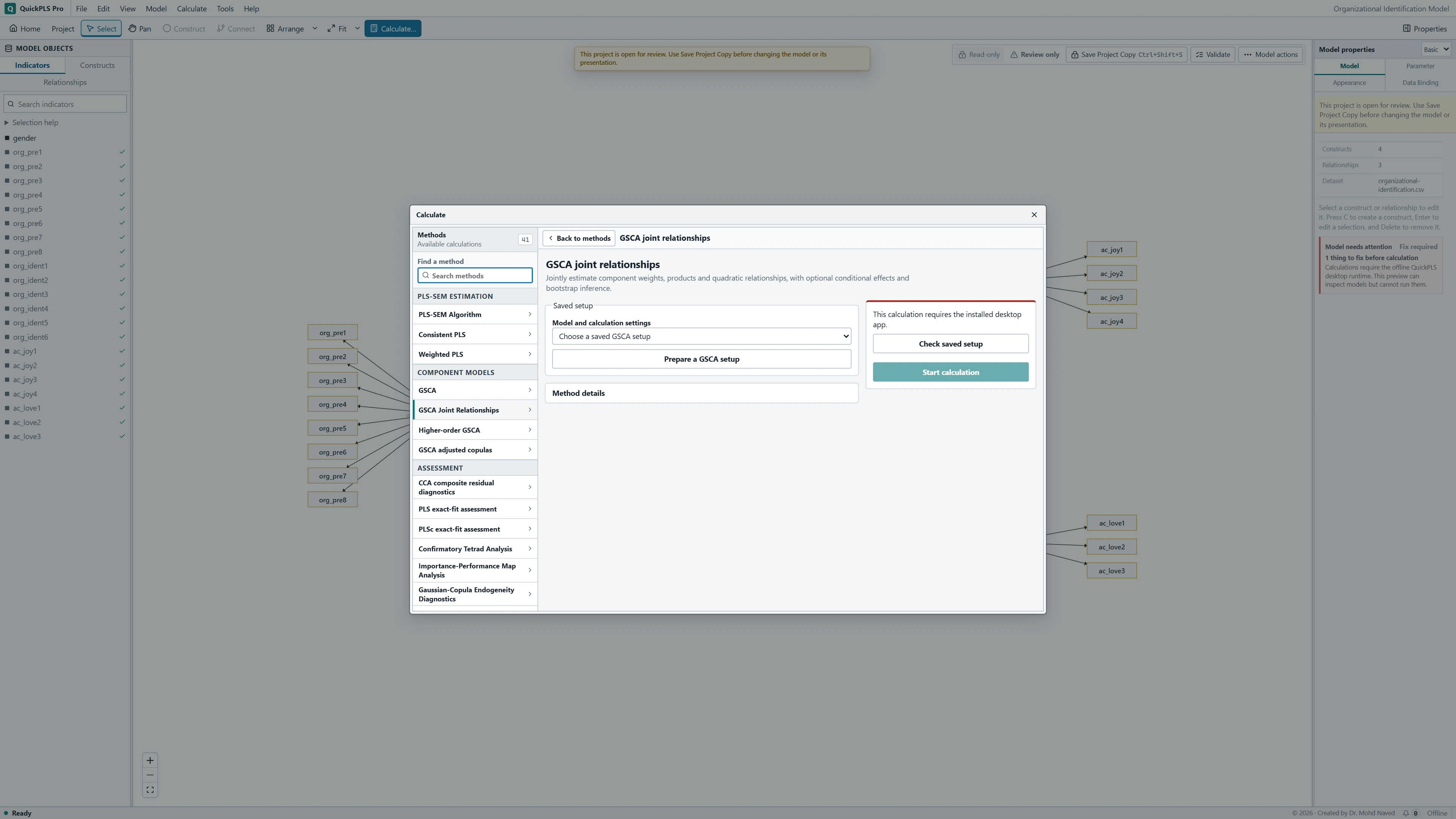
Click Calculate… and select GSCA Joint Relationships. Click Prepare a GSCA setup, then choose your Saved base model and enter a New setup name.
Add terms and evaluation points
Under Joint relationships, click Add relationship, then choose Predictor, Second predictor / moderator and Outcome. Use the same predictor in both predictor fields for a square. Under Conditional effects and simple slopes, click Add probe and enter a value for every component used in the products.
Save the setup and calculate
Choose an Interval method under Inference. Click Preview setup, review the terms and probes, then Save new setup and Use saved setup. Back in the calculation screen, use Check saved setup and Start calculation. After completion, click Open Results.
Read a changing slope from the matching result
In Results, select the completed joint run. Use Search result outputs to find Joint GSCA fit, Component scores, and Conditional effects and simple slopes. Start with convergence and the score ranges, then read the slope at each named probe. Conditional effects at specified probes plots these effects; it is not a plot of predicted Satisfaction.
Read the main, squared and product coefficients as parts of one equation. An interval for a conditional slope must come from that same joint calculation. An interval from regression on scores exported from an earlier fit answers a different question.
On a small screen, swipe the table sideways to see every column.
| Output | How to read it | What to check |
|---|---|---|
| Joint coefficients | Linear, product and quadratic terms in the same estimated specification. | Report the main relationships and how the variables were centred. |
| Conditional curves / effects | The relationship evaluated at the stated predictor or moderator values. | Curves outside the data range are extrapolation. |
| Raw-case refit intervals | Uncertainty from the specified full-refit procedure. | Use the fit measures provided for the nonlinear model; ordinary linear fit formulas may not apply. |

Describe the pattern, not just the product coefficient
A useful result statement names the predictor, the outcome and the values of the other variables: for example, whether Quality has a stronger association with Satisfaction at lower or higher Trust. The example below explains why the entire equation matters.
Illustrative example, not a software benchmark
When a predictor has both a quadratic term and an interaction, its slope can vary with its own value and with the moderator. One overall statement about the effect of X hides these differences. Report slopes at the values you evaluated and explain why you chose those values.
Practice: Quality, Trust and diminishing returns
Download research-workshop.csv and use the Quality, Trust, Satisfaction and Loyalty indicator blocks. Keep the three main paths: Quality → Satisfaction, Trust → Satisfaction and Satisfaction → Loyalty. The last path lets you explore how a changing Quality relationship carries through Satisfaction to Loyalty.
The planned extension contains Quality squared and Quality × Trust in the Satisfaction equation. The square asks whether the Quality relationship bends. The product asks whether Trust changes that relationship. Record these questions before inspecting the added terms' significance.
Use the indicators to form GSCA components. The supplied quality_mean and trust_mean columns are simple observed averages. Multiplying those columns would create a different analysis from multiplying component scores estimated by the joint GSCA procedure. The arithmetic later in this guide is a teaching example, not an answer key for this CSV.
Add the square, product and probes
Save the base model
Check the four indicator blocks and three main paths, then save the model. Keep a record of the cases retained after missing values are handled.
What you should see: The base model contains the intended components and paths.
How to read it: Save it so the joint term has an identifiable source model.
Prepare the saved setup
Open Calculate… → GSCA Joint Relationships → Prepare a GSCA setup. Select the Saved base model and give the setup a name that identifies the planned square and interaction.
What you should see: The saved GSCA relationship setup names the correct model.
How to read it: Confirm it before adding terms.

GSCA Joint Relationships settings in QuickPLS. Select your own dataset and model, then use the choices described in the steps. Enter the Quality square
Under Joint relationships, click Add relationship. Choose Quality for Predictor, Quality again for Second predictor / moderator, and Satisfaction for Outcome. The repeated predictor defines the square. Click Add relationship again and use Quality, Trust and Satisfaction for the product.
What you should see: The Quality squared term belongs to the intended outcome equation.
How to read it: Its linear constituent must remain in that equation.
Enter complete probes
Under Conditional effects and simple slopes, click Add probe. Each probe needs both a Quality value and a Trust value. For this exercise examine Quality at -1, 0 and 1 and Trust at -1, 0 and 1, using separate probes for the combinations you intend to interpret. Later check that the fitted cases support them.
What you should see: Each probe specifies the values needed by the relationship.
How to read it: An incomplete probe cannot define a conditional effect.
Choose the uncertainty calculation
Under Inference, choose Point estimates only, Percentile, Bias-corrected and accelerated (BCa), or Studentized (nested bootstrap). For bootstrap inference record Bootstrap draws, Confidence level (%), Test alternative, Seed and Workers. Studentized inference also needs Inner draws per usable outer draw (odd). Open Optimizer and starting weights only if you need to review numerical settings.
What you should see: The chosen uncertainty procedure and draw settings are recorded.
How to read it: Use full-model uncertainty when that is the requested target.
Preview, save and inspect
Click Preview setup. Check both main paths, the square, the product and every probe before Save new setup. Click Use saved setup, Check saved setup and Start calculation. Open Results and examine fit and convergence before interpreting the conditional effects.
What you should see: The preview and completed output identify the squared term and probe effects.
How to read it: Read the slope over the observed range before describing the curve.
Work out what the square and interaction mean together
Use this hypothetical equation: Satisfaction = intercept + 0.40 Quality + 0.30 Trust - 0.10 Quality squared + 0.20 Quality × Trust. Its local slope for Quality is 0.40 - 0.20 Quality + 0.20 Trust. A local slope describes the change in the fitted outcome near the stated predictor values.
At Trust = 0, that slope is 0.60 when Quality = -1, 0.40 when Quality = 0, and 0.20 when Quality = 1. The negative square coefficient makes the curve bend downward, but Quality still has a positive slope at all three points. At Trust = 1 and Quality = 1, the slope is 0.40 because the interaction also contributes.
A turning point occurs where the slope becomes zero. Here it is Quality = 2 + Trust. Check for cases near that combination of Quality and Trust before describing it as a supported turning point. None of these hypothetical numbers are measured results from the practice file.
On a small screen, swipe the table sideways to see every column.
| Output | Hypothetical example | Interpretation |
|---|---|---|
| Joint coefficients | Linear Quality 0.40; Quality squared -0.10; product 0.20 | Read all terms in the same equation. |
| Conditional derivative | 0.40 - 0.20 Quality + 0.20 Trust | The local slope changes with both Quality and Trust. |
| Conditional curve | Downward curvature at a stated Trust value | A curve is conditional on the other terms being held fixed. |
| Recursive effects | Downstream effects through Satisfaction to Loyalty | Follow the defined local slope and downstream paths when interpreting the indirect change. |
| Fit and convergence | Joint objective and model-specific diagnostics | Use the joint model's diagnostics; linear formulas do not supply nonlinear GFI and SRMR. |
| Intervals | Matching full raw-case refits | Do not use uncertainty from a fixed-score OLS fit as if it refitted GSCA. |
Understand the units behind each probe
The joint procedure centers indicators and component scores and scales them using population standard deviations, with the number of analyzed cases, N, rather than N−1 in the denominator. It includes explicit intercepts. It forms products from those normalized component scores without separately standardizing the products. A probe at 0 is on this centered component scale.
Historical linear GSCA uses sample standard deviations. In addition, the joint model estimates weights while fitting the nonlinear relationships. These differences mean that regression on previously exported linear GSCA scores is not a numerical reproduction of the joint procedure.
A full raw-case bootstrap samples cases and refits the model before calculating the same conditional quantities. Read the interval for the slope at Quality = 1 and Trust = -1 if that is your research question. The square coefficient's interval alone cannot answer it.
If the shape or calculation looks wrong
First check the saved equation and the probe values. Then look for nearly constant products, redundant predictors or too little data around a probe. Correct a coding or specification error before drawing conclusions; keep an unsupported theoretical pattern as an honest finding. The checks below help separate these situations.
On a small screen, swipe the table sideways to see every column.
| Symptom | Check | Reasonable action |
|---|---|---|
| A negative square coefficient is reported as an everywhere negative effect | The linear term and local derivative | Calculate and describe slopes at supported values. |
| The turning point lies beyond the scores | Observed score ranges and the combinations of predictor values represented in the sample | Treat it as extrapolation; do not recommend that level as an observed optimum. |
| The joint model disagrees with regression on exported scores | Whether weights were refitted and scales matched | Compare like procedures, or report the two-step model separately. |
| The optimizer or a bootstrap draw fails | Rank deficiency, near-constant products and starting weights | Inspect model complexity and valid alternatives before interpreting intervals. |
| Linear-model fit values are expected for the curve | The available nonlinear output definitions | Report the supported joint diagnostics and leave unavailable fit measures absent. |
Check whether the pattern is stable
Keep the planned linear model and the planned nonlinear extension as separate specifications. Compare the size and shape of the fitted relationship and its uncertainty. Retain the main paths behind a product; removing them changes what the product coefficient means.
Examine a small grid within the observed ranges. A high Quality value and a low Trust value may each occur in the data while almost never occurring together. Mark such combinations as weakly supported when you explain the curve.
If convergence requires another starting vector, compare the final objectives and scores after aligning their signs. Choose a numerically stable solution rather than the most attractive curve. Better fit to the current sample does not establish better prediction for new cases; assess prediction separately when that is the goal.
Write the equation, slopes and data range
Methods example: We fitted Quality and Trust main effects, a Quality squared term and a Quality-by-Trust interaction in the Satisfaction equation. Component scores used population-standard-deviation scaling. We evaluated conditional slopes within the observed score range and used a bootstrap that refitted the complete indicator-based model. Add your actual draws, interval method, confidence level, seed and convergence information.
Results example: The hypothetical linear Quality, quadratic Quality and interaction coefficients were 0.40, -0.10 and 0.20. At mean Trust, the Quality slopes at -1, 0 and 1 were 0.60, 0.40 and 0.20. The turning point changed with Trust and was interpreted only where observations supported the combination. Replace these illustrative numbers with your saved results; they are not CSV answers.
| Item | Required report detail |
|---|---|
| Equation | All main, squared and product terms |
| Coordinate scale | Component scores scaled using population standard deviations, with raw products formed from those scaled scores |
| Conditional estimates | Probe grid, local slopes and matching intervals |
| Numerical assessment | Objective, convergence and initialization |
| Data support | Analysed cases and supported score range |
| Uncertainty | Full-refit procedure, counts and failures |
Check that you can explain the result
- Write the full Satisfaction equation and identify what each term contributes.
- Work out the Quality slope at three supported combinations of Quality and Trust.
- Find the turning point, then explain whether the sample contains cases near it.
- Explain why the interaction coefficient alone cannot describe every Quality slope.
- Describe what is refitted in joint GSCA and what would remain fixed in regression on exported scores.
Make the changing relationship easy to follow
- Write the complete equation, including the main paths behind every square and product.
- State the indicator and component scaling, the probe values, and whether observations support those combinations.
- Report the joint objective, convergence checks and the full-refit bootstrap settings, including failed fits.
- Give the conditional slopes and their matching intervals. Explain the practical difference between the chosen probes.
Keep the conclusion within the fitted model
A nonlinear result describes the equation you fitted on the cases available. A turning point outside those cases is an extrapolation, meaning a prediction beyond the observed range. It cannot establish the best level of a predictor in practice.
Use the fit measures supplied for this joint model. Ordinary linear-model GFI or SRMR formulas do not become valid merely because the nonlinear calculation returns coefficients.