 QuickPLS
What the method does
An endogeneity concern arises when a predictor is associated with the equation error. A Gaussian-copula approach uses a transformation of the predictor distribution as an additional regression term. In this workflow, the diagnostic concerns GSCA score regressions. Its identification assumptions and data distribution matter; adding a term does not establish that every source of bias has been removed.
Copula transform: c(X) = Φ⁻¹(F̂X(X)). Diagnostic equation: Y = b₀ + bX + γc(X) + ε.
F̂X maps predictor values to empirical cumulative probabilities; Φ⁻¹ maps those probabilities to normal quantiles. The expression explains the copula idea. Adjusted constructions account for other predictors as specified by the method. Read the focal coefficient and copula coefficient γ together.
Data and analysis in QuickPLS
Use a GSCA model with the relevant predictor scores and a defensible reason to question exogeneity. Inspect predictor distributions and dependence among predictors.
QuickPLS provides adjusted-copula settings and the associated score-regression tables. Compare the original and adjusted equations for your model and retain the diagnostics explaining whether the calculation is usable.
Follow a worked example
The following example shows the data, settings and decisions for one analysis. Use the linked practice files to follow it. For your own study, keep the procedure and choose the variables, model and settings that fit your research question.
Download research-workshop.csv to begin. It contains 360 rows and 31 columns. The example below identifies the variables to use, their roles and any rows to exclude; not every column is an analysis variable.
Would a possible endogeneity problem change the GSCA result?
Suppose Satisfaction predicts Loyalty, but an unmeasured customer characteristic may influence both. Satisfaction may then be related to the unexplained part of the Loyalty equation. This is an endogeneity concern, and it can distort the estimated relationship.
GSCA adjusted copulas adds controls derived from the distributions of specified predictors. It first estimates GSCA scores, then fits the adjusted score regressions. Use it to examine a stated endogeneity concern under the method's assumptions. The analysis does not jointly re-estimate the GSCA component weights with the copula controls.
Save the scoring setup and identify the affected equation
Prepare a saved point-only GSCA scoring setup. Decide which equation needs adjustment and which predictors are treated as endogenous, meaning potentially related to its unexplained part. Also identify the exogenous predictors, those treated as unrelated to that unexplained part, used for conditioning. Their roles belong to a particular equation, not automatically to the whole model.
Keep the point-only scoring setup and its dataset identifiable before opening the adjustment. Inspect scoring setup must resolve to the Quality, Trust, Satisfaction and Loyalty model described below, not a score file or a result from a different model.
Choose a saved scoring setup and add controls
Inspect the source setup
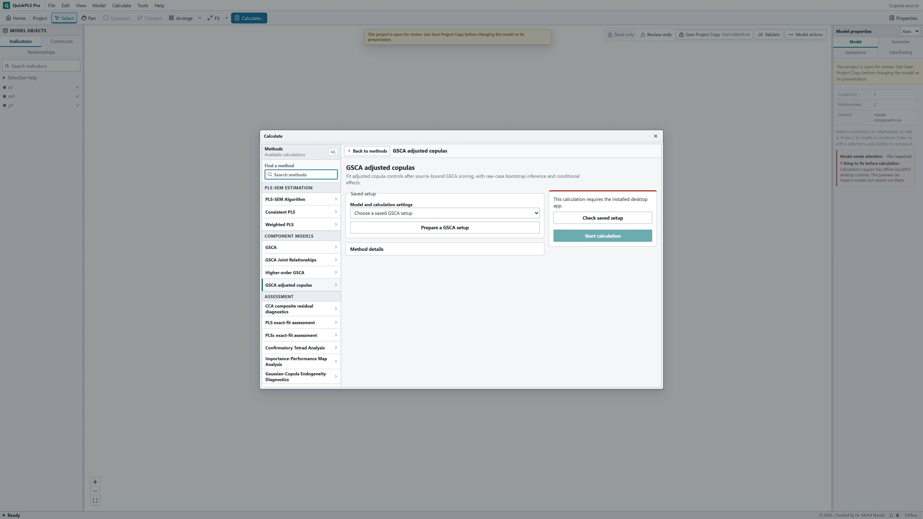
Open Calculate… → GSCA adjusted copulas → Prepare a GSCA setup. Choose the Saved GSCA scoring setup and click Inspect scoring setup. Enter a New setup name.
Classify the predictors in each affected equation
Under Adjusted Gaussian copula controls, select Add controls to the intended outcome equation. Use each predictor's dropdown to choose Continuous endogenous, Continuous exogenous or Discrete exogenous as justified by its role and measurement.
Save and run the adjustment
Choose the Inference settings. Preview setup, review the equation-specific controls, Save new setup and Use saved setup. Then Check saved setup and Start calculation. Click Open Results and read the adjusted regression with the scoring and inference diagnostics.
Read the adjusted relationship alongside the original
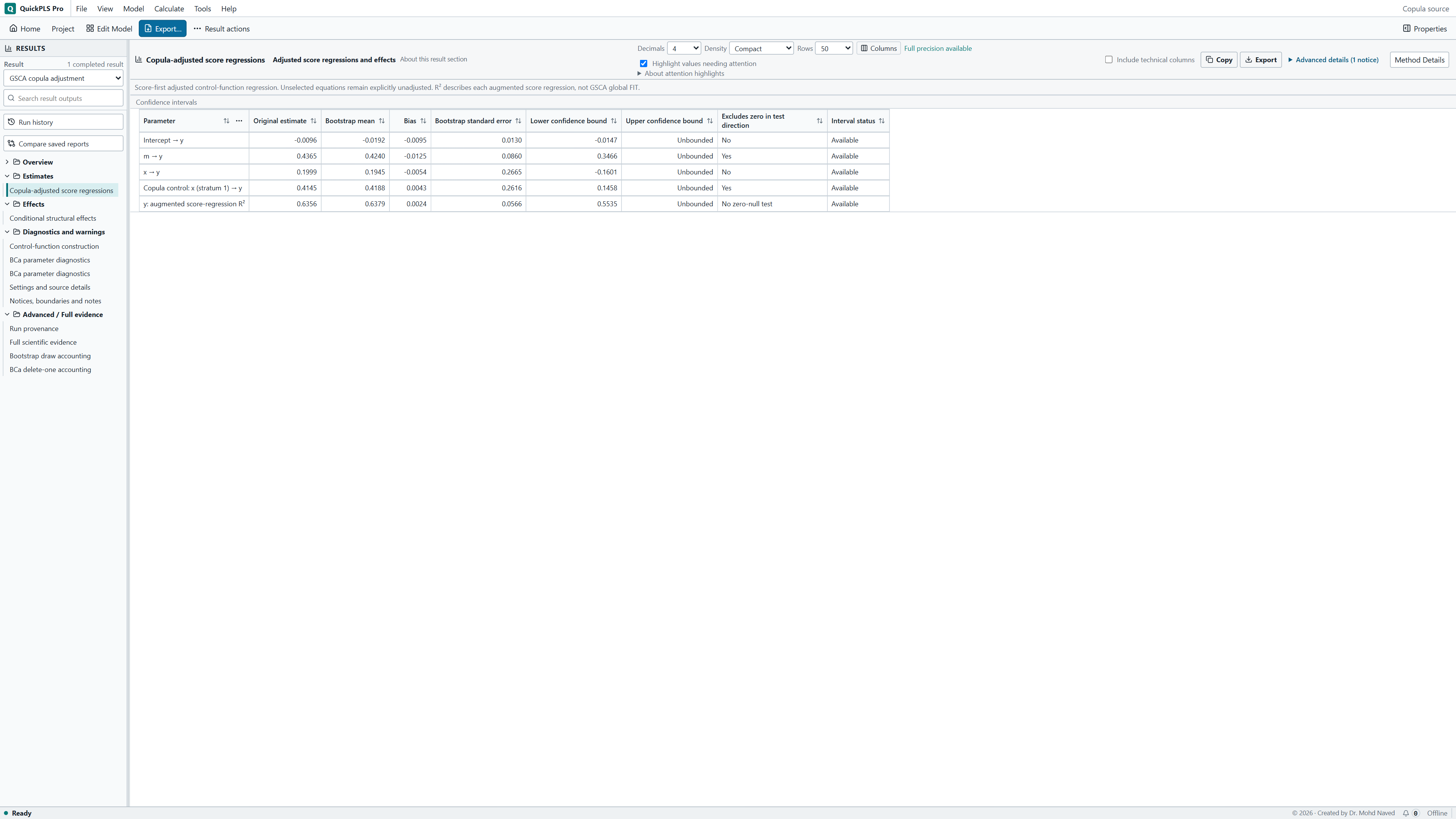
In the completed result, find Copula-adjusted score regressions. Compare the affected structural coefficient with the unadjusted relationship using matching scores and sample definitions. Check the copula controls and regression diagnostics before explaining a change as substantive.
If requested and available, Conditional structural effects gives the defined direct, indirect and total effects. These structural derivatives hold the copula controls fixed. They do not describe what happens when the empirical ranks used to construct the controls are also changed.
On a small screen, swipe the table sideways to see every column.
| Output | How to read it | What to check |
|---|---|---|
| GSCA model used for scoring | The component definitions underlying the adjustment. | If the score model changes, calculate and identify a new analysis result. |
| Adjusted coefficients / controls | Relationships estimated with the specified copula control terms added. | Changed coefficients do not establish removal of all bias. |
| Uncertainty from scoring and adjustment | Intervals calculated by repeating the specified scoring and adjustment steps. | Do not substitute uncertainty from an unrelated score regression. |
Ask what changed and whether the adjustment is credible
An adjusted coefficient is useful only when the predictor roles, distributional assumptions and numerical diagnostics support its interpretation. A large change deserves explanation; a small change does not prove that endogeneity was absent.
Illustrative example, not a software benchmark
Two programs can both report a copula analysis while performing different calculations. One may hold scores fixed while another repeats a scoring stage. Before comparing their numbers, check how each obtains the scores and refits the model. The shared name alone cannot establish numerical equivalence.
Practice: examine Satisfaction in the Loyalty equation
Use the Quality, Trust, Satisfaction and Loyalty indicator blocks in research-workshop.csv. Keep Quality → Satisfaction, Trust → Satisfaction and Satisfaction → Loyalty. First prepare a point-only GSCA scoring setup for this model.
For the exercise, treat Satisfaction as a continuous endogenous predictor in the Loyalty equation. The teaching question is whether its relationship with Loyalty changes after a supported copula adjustment. In your own study, justify that concern and the role of any conditioning predictors before running the analysis.
Use GSCA scores derived from the indicator blocks, not the supplied observed mean columns. The hypothetical coefficient comparison later in the guide explains how to discuss a result; it is not a checked answer from this file.
Set the predictor roles where they apply
Keep a point-only scoring source
Save the intended GSCA scoring setup without bootstrap inference. For linear GSCA, choose Estimation → Point estimates. For a joint GSCA setup, choose Inference → Interval method → Point estimates only. The setup must specify the measurement model, component scale and structural relationships used to generate scores.
What you should see: A saved point-only GSCA source result is available.
How to read it: Keep its original coefficients for the later comparison.
Open and inspect it
Choose Calculate… → GSCA adjusted copulas → Prepare a GSCA setup. Select the Saved GSCA scoring setup and click Inspect scoring setup before configuring the adjustment.
What you should see: The preparation identifies that source result.
How to read it: Correct an unintended dataset or model before proceeding.

GSCA adjusted copulas settings in QuickPLS. Select your own dataset and model, then use the choices described in the steps. Choose the Loyalty equation
Under Adjusted Gaussian copula controls, find Equation: Loyalty and select Add controls to Loyalty. Set Satisfaction to Continuous endogenous. Classify other predictors only according to their justified role in this equation.
What you should see: The Loyalty equation and its questioned predictors are selected.
How to read it: The copula terms must correspond to the equation being diagnosed.
Check discrete classifications
Use Discrete exogenous only for a supported categorical predictor represented by a single original observed indicator. A multi-item component does not become an observed categorical variable merely because its scores have repeated values.
What you should see: Discrete or continuous classifications match the observed predictors.
How to read it: Incorrect classifications change the adjustment assumptions.
Choose effects and uncertainty
For a linear source, select Include recursive direct, indirect and total structural effects if those effects answer your question. A joint source inherits its products; review its supported probes. Under Inference, set the interval method and, when applicable, draws, confidence, alternative, seed and workers.
What you should see: Requested effects and uncertainty are recorded.
How to read it: Interpret only the effect definitions actually calculated.
Preview and compare the results
Click Preview setup, review the roles and source definition, then Save new setup and Use saved setup. Use Check saved setup and Start calculation. Click Open Results, then inspect Copula-adjusted score regressions, analysed cases, control diagnostics and any requested Conditional structural effects.
What you should see: The completed output distinguishes original predictors and adjustment terms.
How to read it: Check distribution and fit diagnostics before comparing coefficients.
A changed coefficient is not a measured amount of bias
Suppose the unadjusted Satisfaction → Loyalty coefficient is 0.50 and the adjusted coefficient is 0.30. This tells you that the fitted relationship changed under the stated adjustment. It does not establish that exactly 0.20 of bias was removed.
Read the adjusted 0.30 with its interval, the predictor distribution and the control diagnostics. If the original predictor and its copula control are almost redundant, the estimate can become unstable. More bootstrap draws do not create the missing information needed to distinguish them.
The procedure fits GSCA scores first, then adjusted regressions. Its regression R² describes the augmented equation and is not the original GSCA FIT statistic. When structural effects are reported, the copula controls remain fixed while the structural derivatives are evaluated.
On a small screen, swipe the table sideways to see every column.
| Output | Hypothetical reading or question | Interpretation |
|---|---|---|
| Scoring source | Which GSCA model supplied the components? | Its measurement and score scale remain part of the analysis. |
| Adjusted structural coefficient | 0.30 compared with unadjusted 0.50 | Shows sensitivity to the chosen adjustment; it does not establish that bias has been removed. |
| Copula controls | Which regressor and equation generated each term? | A control is not an additional substantive construct. |
| Augmented regression R-square | Variation fitted by the adjusted equation | Keep it distinct from base GSCA FIT. |
| Conditional effects | Slopes calculated while holding the fitted control terms fixed | Use the stated derivative definition and supported probes. |
| Full-refit intervals | Scoring and controls rebuilt from raw cases | Errors from a regression conditional on one set of scores omit uncertainty from estimating scores and rebuilding controls. |
Investigate instability before interpreting a change
If the adjusted coefficient changes sharply or becomes imprecise, inspect the predictor distribution, ties, category counts and control collinearity. Verify the scoring source and equation-specific roles before treating the shift as a research finding. Use the checks in the table to choose a defensible next step.
On a small screen, swipe the table sideways to see every column.
| Symptom | Check | Reasonable action |
|---|---|---|
| The adjusted coefficient changes dramatically | Control collinearity, regressor distribution and original model | Investigate identification and substantive assumptions before calling the adjusted value correct. |
| A regressor role is wrong in one equation | Equation-specific endogenous and exogenous assignments | Correct the particular equation; avoid applying one role automatically everywhere. |
| Controls or refits become singular | Ties, sparse categories, score variation and rank checks | Report the limitation and reconsider a supported specification; do not discard failed draws quietly. |
| Intervals from a fixed-score regression seem easier to obtain | Whether GSCA scores and controls were regenerated | Use refits that repeat scoring and control construction when reporting uncertainty in the complete analysis. |
| A nonlinear effect is called the derivative of the ranks | The structural-part derivative definition | Interpret it with fitted controls held fixed and state that convention. |
Compare justified assumptions openly
Compare the unadjusted model with the adjustment you planned. If another endogeneity classification is scientifically plausible, label it as a sensitivity analysis and explain the different assumption. Do not search across classifications for the smallest p-value.
A full raw-case bootstrap must repeat the scoring and control construction before refitting the adjusted equation. A regression bootstrap that holds the original component scores and copula controls fixed omits those sources of variation.
If conclusions depend heavily on a fragile distribution or a sparse category, report that dependence. Better measurement, time ordering or a design that addresses the suspected omitted cause may be more useful than further tuning of the same data.
Explain the scoring and adjustment as separate steps
Methods example: We estimated GSCA component scores from the specified indicator model, then applied adjusted Gaussian copula controls to the Loyalty equation with Satisfaction treated as continuous endogenous. We documented the conditioning roles, retained sample and score scale. The uncertainty procedure repeated the complete raw-case scoring and adjustment process. Replace these descriptions with your actual settings.
Results example: The hypothetical Satisfaction → Loyalty estimate changed from 0.50 to 0.30. We interpreted this as sensitivity to the stated adjustment, with the corresponding interval and diagnostics, rather than as proof that a known amount of bias had been removed. These numbers illustrate the wording and are not results from the practice data.
| Item | Report |
|---|---|
| Scoring analysis | Named GSCA setup, blocks, scales and common cases |
| Affected equation | Loyalty with Satisfaction designated potentially endogenous |
| Roles and assumptions | Continuous/discrete and endogenous/exogenous assignments |
| Estimates | Unadjusted and adjusted structural coefficients plus control terms |
| Uncertainty | Full scoring-and-control refits, interval method and failures |
| Interpretation | Identification assumptions and any controls-held-fixed derivative convention |
Check that you can explain the adjustment
- Name the outcome equation and explain why one of its predictors may be endogenous.
- Distinguish the GSCA scoring step from the adjusted regression step.
- Explain why a change in the coefficient does not measure the exact amount of bias removed.
- Identify the distributional and collinearity checks needed before interpreting the adjusted path.
- Explain what stays fixed when conditional structural effects are calculated and what is refitted in a raw-case bootstrap.
Describe exactly what was adjusted
- Identify the saved GSCA scoring procedure, analyzed cases and selected outcome equations.
- Explain the endogenous, exogenous and discrete predictor roles and the substantive reason for each choice.
- Report the original and adjusted structural estimates, the copula controls and their uncertainty.
- State that scoring precedes adjusted regression, and describe full raw-case refits and the fixed-control convention for structural effects.
Use the adjustment as part of the research design
An instrument-free procedure does not remove the need for assumptions. The observed predictor distributions and the specified conditioning relationships must support the adjustment. Near-normal scores, extensive ties or redundant controls can leave little information for separating the copula term from the original predictor.
The adjustment does not turn observational data into an experiment. If reverse causality, omitted causes or weak identification remain plausible, discuss those issues and consider a stronger design rather than presenting the adjusted path as established causality.
When comparing software results, match the GSCA scoring, score scale, adjustment and refitting choices before comparing coefficients.