 QuickPLS
What the method does
Generalized structured component analysis (GSCA) forms components from observed indicators and estimates a model through a least-squares criterion. Alternating updates estimate the component weights and model coefficients. Its overall fitting criterion differs from the sequence used by ordinary PLS, so fit summaries and estimates should be interpreted as GSCA results.
Components: Γ = XW. Least-squares criterion: minimise ‖ZV − ZWA‖².
X contains observed indicators and W contains component weights. In the compact GSCA expression, Z is the data matrix, V selects the variables to be reproduced and A contains the model coefficients. The squared residual norm measures the discrepancy the algorithm minimises.
Data and analysis in QuickPLS
Use numeric observations in rows, indicators in columns, and a specified component model. Check coding, missingness and the number of usable cases before fitting.
QuickPLS provides GSCA estimation, component weights, structural paths and fit information. Build your own model or follow the practice specification below, then inspect convergence before interpreting the result.
Follow a worked example
The following example shows the data, settings and decisions for one analysis. Use the linked practice files to follow it. For your own study, keep the procedure and choose the variables, model and settings that fit your research question.
Download research-workshop.csv to begin. It contains 360 rows and 31 columns. The example below identifies the variables to use, their roles and any rows to exclude; not every column is an analysis variable.
Choose GSCA to fit component scores and their relationships together
Suppose you want to represent Quality, Trust and other concepts as weighted combinations of their measurements. Each combination forms a component score. Generalized structured component analysis, or GSCA, estimates those scores and their relationships together.
GSCA uses one joint objective: a quantity that measures discrepancies across the measurement and structural parts of the model. The calculation searches for weights and coefficients that make this quantity smaller. That objective differs from ordinary PLS and from a common-factor model.
Choose the method because this component interpretation and joint fit suit the study. Define each group of indicators and how its score will be scaled. When comparing software, match these choices before comparing the reported numbers.
Before interpreting a path, check convergence, meaning that the repeated estimation steps reached a stable solution. Then assess fit and, when needed, use the corresponding GSCA refits to describe uncertainty.
Practise with Quality, Trust, Satisfaction and Loyalty
Use research-workshop.csv. Assign Quality, Trust, Satisfaction and Loyalty their three matching indicators, then draw Quality → Satisfaction, Trust → Satisfaction and Satisfaction → Loyalty. Keep case_id, group, weight and the supplied arithmetic means outside the indicator assignments.
Assign quality_1, quality_2 and quality_3 to Quality; trust_1, trust_2 and trust_3 to Trust; satisfaction_1, satisfaction_2 and satisfaction_3 to Satisfaction; and loyalty_1, loyalty_2 and loyalty_3 to Loyalty.
Use reflective blocks for this first exercise so you can compare the component weights with the measurement loadings. Reflective means that the indicators are treated as expressions of the concept represented by the component.
GSCA fits the measurement and structural relationships together by minimising their combined squared discrepancies. Squaring makes positive and negative discrepancies contribute rather than cancel. A factor model fitted to reproduce covariances has a different interpretation and objective.
The data were invented for learning. They give you a manageable connected model rather than evidence that the named constructs have been validated. Use this linear model as a starting point before attempting the separate joint-relationship, higher-order or adjusted-copula extensions, which introduce their own choices and assumptions.
Define the components, indicators and paths
For each component, identify the measured columns that should form its score. Specify the structural paths, the proposed relationships between components, for the selected dataset.
Check score normalisation, meaning the convention used to set the score's scale. Decide what each block represents before choosing a confidence-interval method. A well-labelled component is easier to interpret than a collection of indicators chosen only because they produce attractive paths.
Run GSCA and check that estimation finished successfully
Select the saved workshop model before opening GSCA. The first calculation uses Point estimates; save a separate Bootstrap inference result when you are ready to assess uncertainty.
Open GSCA for the component model
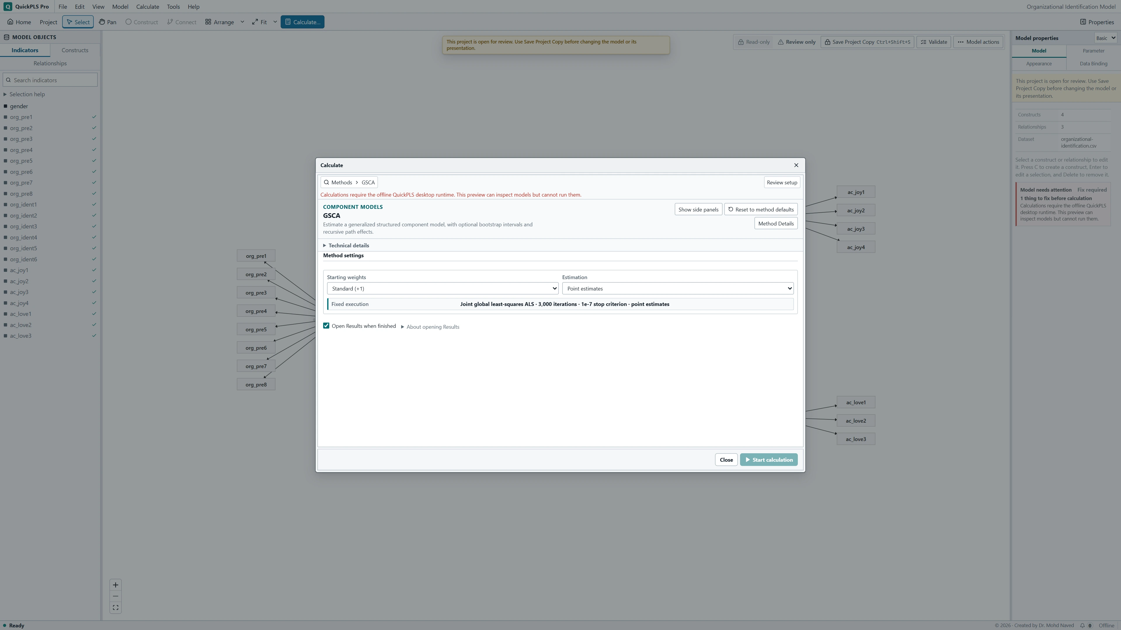
Click Calculate…, type GSCA into Find a method and select GSCA. This guide uses the linear GSCA row, not GSCA Joint Relationships, Higher-Order GSCA or GSCA adjusted copulas.
Choose the initial calculation
Set Starting weights → Standard (+1) and Estimation → Point estimates. Fixed execution shows the algorithm's convergence settings; they are not editable GSCA fields. For intervals, change Estimation to Bootstrap inference, then select Interval method and the additional bootstrap settings.
Start and inspect convergence
Review Readiness, leave Open Results when finished selected and click Start calculation. In Results, open Model fit → Model fit and convergence. Check Converged, ALS iterations, Objective and Analyzed observations before reading the coefficients. Estimates contains Component weights, Measurement loadings, Structural path coefficients and Endogenous construct R².
Fit the linear workshop model
Check the component model
Check the numeric indicators, variation and missing values. Confirm the three stated paths and avoid structural feedback loops. Every component in this initial GSCA model must take part in the structural model. Keep case_id, group and weight outside the indicator blocks.
What you should see: The intended indicator blocks and paths are visible.
How to read it: Keep them unchanged for the first GSCA calculation.
Find the linear GSCA row
With the model and dataset open, click Calculate… and use Find a method to select GSCA. The linear procedure standardises the indicators and uses cases complete on every required variable. There is no Result data or Missing data dropdown for this GSCA setup.
What you should see: GSCA is selected for the intended model.
How to read it: Confirm the data and method before entering numerical settings.

GSCA settings in QuickPLS. Select your own dataset and model, then use the choices described in the steps. Set the starting weights
Choose Starting weights → Standard (+1). For a later starting-value comparison, choose Individual indicator weights. A field appears for every model indicator. Enter finite values with at least one nonzero value in each construct. Reset current model weights to +1 restores the current indicator list's starting values.
What you should see: The stated calculation settings appear in the setup.
How to read it: Resolve Readiness messages before starting.
Choose point estimates or bootstrap inference
Choose Estimation → Point estimates for the first fit check. For intervals, choose Estimation → Bootstrap inference. Review Bootstrap draws, Confidence level (%), Interval method, Test direction, Seed and Workers. Studentized (nested bootstrap) reveals Inner draws per outer fit. If the question needs indirect and total effects, set Path effects → Include direct, indirect and total effects.
What you should see: The setup shows Point estimates or the selected bootstrap inference, with its requested effects.
How to read it: Choose inference only when uncertainty is required.
Read the fixed settings and run
The Fixed execution line reports the 3000-iteration limit and 1e-7 stop criterion. These are fixed for this linear GSCA route; there are no editable Maximum iterations or Stop criterion fields here. Review Readiness and click Start calculation. Afterwards, open Model fit → Model fit and convergence to check the convergence status, iterations, objective and analysed sample.
What you should see: The saved result reports convergence, iterations, objective and analysed cases.
How to read it: Resolve a failed or incomplete fit before interpreting coefficients.
Read the model and its uncertainty together
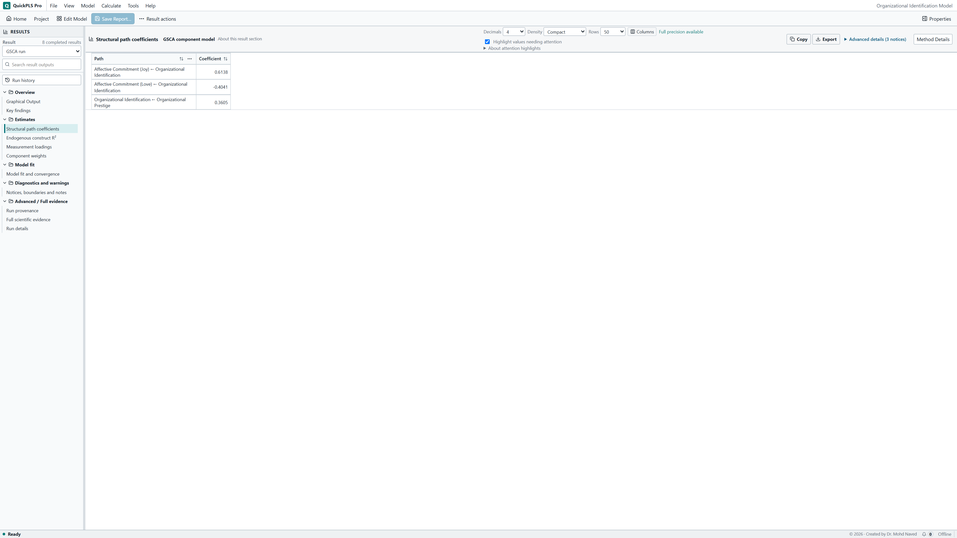
Under Estimates, open Component weights, Measurement loadings, Structural path coefficients and Endogenous construct R². Read the separate FIT measures in Model fit and convergence. For a bootstrap run, open Inference → GSCA bootstrap intervals and read Interval status as well as Lower bound and Upper bound. Use the matching result when reporting uncertainty.
What you should see: Component weights, loadings, paths and R² identify the intended constructs.
How to read it: For a bootstrap run, read interval status and bounds from the same result.
Read weights, loadings and paths as different quantities
Open Estimates → Component weights to see how the score is built. Then open Estimates → Measurement loadings to see how each indicator relates to that score. A small weight and a large loading need not contradict each other.
Open Estimates → Structural path coefficients for relationships between components. Estimates → Endogenous construct R² reports the fitted explained variation for outcomes with incoming paths. When requesting recursive effects in a bootstrap run, choose Path effects → Include direct, indirect and total effects in the setup first.
Open Model fit → Model fit and convergence before interpreting paths. Read Converged, ALS iterations, Objective, Analyzed observations and Omitted observations. Coefficients alone are not enough when the numerical fit needs investigation. Use Search result outputs if a table is not visible.
Select the workshop result in the Result dropdown before reading fit or paths. Keep its analysed case count, convergence and objective with its coefficients so that every reported value belongs to the same calculation.
On a small screen, swipe the table sideways to see every column.
| Output | How to read it | What to check |
|---|---|---|
| Weights and loadings | How observed indicators contribute to, and relate to, their components. | Keep the score normalization explicit. |
| Paths and recursive effects | Direct and supported indirect relationships in the component model. | A causal interpretation of an indirect coefficient still needs justification from the study design. |
| Objective, fit and convergence | Whether fitting reached a stable solution (converged), and which measure of disagreement between model and data it minimised. | Do not interpret coefficients as a successful fit when convergence failed. |
Compare GSCA results under matching definitions
How to read a software comparison
A reflective GSCA model may agree closely with a separately configured reference, while a model containing both reflective and formative blocks may differ. Compare the measurement roles, objective and settings for each case. Combining those discrepancies into one average score would conceal which comparison agreed and which did not. The GSCA benchmark record describes the actual comparisons; this explanation adds no new benchmark result.
Keep the model definition and calculation checks with the result
- Describe the indicators in each component, the structural paths and the score-normalisation convention.
- Report the objective, convergence checks and fit measures that apply to the selected analysis.
- When reporting uncertainty, state the bootstrap interval procedure and the number of usable refits.
Interpret the model that GSCA actually estimated
GSCA uses a component model and its own fitting objective. A coefficient from ordinary PLS or common-factor SEM is not automatically the same quantity under another name.
Use the fit measures available for the selected analysis. GFI and SRMR summarise model fit, but their nonlinear versions are not available for every extension. Do not carry a linear-model formula into a different extension without checking that it applies.
Use each result for the question it answers
Read a component's weights to understand how its score was constructed. Then read its loadings to understand how the indicators relate to that score. Indicators sharing similar information can have different conditional contributions, so a small weight does not by itself make an item useless.
Inspect the whole block before removing an indicator. Its content may matter even when other indicators overlap with it. Deleting it changes what the component represents.
For an arithmetic illustration, suppose Quality → Satisfaction is 0.45 and Trust → Satisfaction is 0.25. These describe their respective associations with Satisfaction after accounting for the other predictor, on the reported component-score scale.
If Satisfaction R-square is 0.50, the fitted predictors explain half of its sample variation under that model. It does not mean 50% of participants were correctly predicted. Performance on new cases needs a separate assessment.
Keep the overall, measurement and structural FIT summaries distinct from an individual outcome's R-square. Read the fit definition for the model you selected rather than treating every output as another score of the same thing.
On a small screen, swipe the table sideways to see every column.
| Output | Question it answers | Example or check |
|---|---|---|
| Component weights | How is each score constructed? | Inspect sign, relative contribution and score normalization. |
| Measurement loadings | How does each reflective indicator relate to its component? | Assess the complete block rather than weight rank alone. |
| Paths and endogenous R-square | Which relationships and explained variation are fitted? | Hypothetical coefficients 0.45 and 0.25; R-square 0.50. |
| Objective and FIT summaries | How well does the joint least-squares representation account for variation? | Keep overall, measurement and structural summaries distinct. |
| GFI and SRMR | What do the supported linear-model fit measures show? | Do not carry linear formulas into nonlinear GSCA automatically. |
| Refit intervals and diagnostics | How uncertain are the named quantities under resampling? | Check usable draws, interval type and unavailable bounds. |
Include uncertainty from estimating the component scores
GSCA estimates the component scores from the sample. To include that step in uncertainty, use raw-case bootstrap refits: each resample rebuilds the model from the sampled indicator rows.
A regression on one exported score table holds those scores fixed. Bootstrapping that regression therefore answers a narrower question and leaves out uncertainty from estimating the earlier scores.
Percentile intervals use the distribution of refitted estimates. BCa, short for bias-corrected and accelerated, also uses fits that leave out one case at a time. Nested studentized intervals use an additional resampling stage within each main sample to estimate uncertainty there.
Those extra calculations can fail for a quantity even when a percentile interval is available. If your selected interval is unavailable, read and report the reason. A different interval method is a separately named analysis, not an automatic replacement hidden in the report.
A component score and its weights can reverse sign while describing the same axis. Refits must be compared with their directions aligned; mixing positive and negative orientations would distort the bootstrap distribution. Keep the direction and scale recorded for exported scores when interpreting them.
Check numerical problems before explaining the paths
If Start calculation is disabled, read Readiness before changing the model. For this linear exercise, check that every component has its indicators and participates in the structural paths. Confirm that no unintended case-weight setting, feedback loop, interaction or higher-order construct has carried into the calculation.
If you changed settings while exploring another method, Reset to method defaults restores GSCA's supplied defaults. Then review Starting weights and Estimation again before running. If individual starts are invalid after changing indicator assignments, use Reset current model weights to +1 or enter a valid value for every current indicator.
After a run, inspect Model fit → Model fit and convergence. A failed fit, a reversed score direction and an unavailable interval are different problems. In a bootstrap result, read Interval status in GSCA bootstrap intervals and the relevant warnings. More draws do not fix an invalid original model or a failed convergence check.
Once the numerical setup is sound, a small path or wide interval can be a valid finding to report. It is not a reason to keep changing starting weights until a preferred coefficient appears.
On a small screen, swipe the table sideways to see every column.
| Symptom | Check | Reasonable action |
|---|---|---|
| The algorithm does not converge | Objective progression, degenerate scores and starting weights | Inspect the specification and starting vector; document a justified alternative initialization. |
| Weights change sign between analyses | Orientation, indicator coding and component direction | Check that the component scores point in the same direction before interpreting a change in the relationship. |
| A formative block has no reflective loading interpretation | The block role and what enters the objective | Assess contribution and definition instead of applying reflective reliability rules. |
| An interval is unavailable | Failed original, delete-one or nested fits and usable counts | Report the reason; do not replace it without naming a separate analysis. |
| Exported-score regression is more precise | Whether scoring was held fixed | Refit GSCA from raw cases when the interval is meant to include uncertainty from estimating the scores. |
See whether a reasonable starting choice changes the solution
Keep the data and model fixed. For a second run, choose Starting weights → Individual indicator weights and enter a reasonable alternative starting vector: one finite value for each indicator, with at least one nonzero value in each construct. Save the result separately.
Compare Converged, Objective and the coefficients after checking that score directions match. Similar answers support stability for those starts. They do not prove that every possible starting vector reaches the same solution.
If two starts produce materially different usable solutions, investigate and report the instability. Changing the indicator set at the same time would make it difficult to tell numerical sensitivity from a different construct definition.
More bootstrap draws can improve the precision of the resampling calculation, but they cannot add information to the original sample or fix an ill-defined component. An initial diagnostic run can reveal failures before a more demanding interval method.
Report the component model, its fit and its uncertainty
For the workshop, a Methods description could read: We estimated a four-component model without structural feedback using GSCA, standardised continuous indicators and shared complete cases. We fitted the measurement and structural relationships jointly. We recorded the starting weights and convergence settings, assessed component weights and reflective loadings, and used raw-case refits for the stated bootstrap intervals.
For the hypothetical example, a Results description could read: Quality and Trust had coefficients of 0.45 and 0.25 for Satisfaction, whose R-square was 0.50. Overall FIT was interpreted separately from the structural R-square and from prediction on new observations.
The numbers in that paragraph are illustrations, not results from the workshop CSV. A completed paper needs the actual estimates, matching intervals, fit and convergence checks. Include failed or unavailable refits and explain any comparison with another starting vector.
| Item | Report |
|---|---|
| Sample and preparation | Analysed count, omissions and standardized input |
| Specification | Indicator blocks, block roles and three structural paths |
| Numerical fit | Initialization, convergence, iterations and objective |
| Measurement | Component weights and eligible loadings |
| Structure | Paths, intervals and endogenous R-square |
| Uncertainty | Interval procedure, requested and usable refits, failures and seed |
Check that you can explain the joint fit
- Explain why a component weight and an indicator loading can differ.
- Match the analysed case count to the complete-case preparation.
- Find the separate measurement and structural fit summaries.
- Compare one alternative starting vector while keeping the model unchanged.
- Explain which uncertainty is left out by a regression on fixed exported scores.