 QuickPLS
What the method does
Gaussian-copula diagnostics add distribution-based terms to an equation containing a potentially endogenous predictor. The method relies on distributional and identification assumptions. It can inform an endogeneity assessment, but it cannot replace a research design or establish that all omitted influences have been controlled.
c(X) = Φ⁻¹(F̂X(X)); Y = b₀ + bX + γc(X) + ε.
F̂X is an empirical distribution function and Φ⁻¹ is the inverse standard-normal distribution. The added term captures the dependence assumed by the copula model. Inspect distribution checks, coefficient changes and uncertainty together.
Data and analysis in QuickPLS
Use an eligible PLS specification with a clearly identified focal predictor and a reason to question exogeneity. Inspect the predictor’s distribution and its dependence on other predictors.
QuickPLS provides the copula setup, augmented-equation estimates and diagnostics. Retain both the original and augmented model results for a transparent comparison.
Follow a worked example
The following example shows the data, settings and decisions for one analysis. Use the linked practice files to follow it. For your own study, keep the procedure and choose the variables, model and settings that fit your research question.
Download research-workshop.csv to begin. It contains 360 rows and 31 columns. The example below identifies the variables to use, their roles and any rows to exclude; not every column is an analysis variable.
Could an omitted cause be affecting a PLS path?
Suppose Quality predicts Satisfaction, but an unmeasured customer characteristic affects both. Quality may be related to the unexplained part of the Satisfaction equation. This is called endogeneity. It can make the fitted path misleading even when the software calculates it correctly.
The Gaussian-copula diagnostic adds a control derived from the selected predictor's score distribution. It lets you inspect how the relationship changes and whether the control contributes under the method's assumptions. It is a diagnostic for a stated concern, not a test that can certify every path as causal.
Choose the questioned path for a reason
Start with a checked PLS model and identify the structural path whose predictor may be endogenous. Write down the possible omitted cause, reverse direction or other reason for concern before selecting focal paths.
Check the predictor's score distribution. The method needs useful distributional information to distinguish the original predictor from its copula control. A score close to normally distributed can make those terms nearly redundant. A significant normality test alone does not guarantee a well-identified adjustment.
Select the focal paths and run the diagnostic
For this exercise, select Quality → Satisfaction as the focal concern. Trust → Satisfaction remains an ordinary predictor in the equation; selecting it as another focal path would add a second endogeneity question.
Open the diagnostic
Click Calculate… and choose Gaussian-Copula Endogeneity Diagnostics. Review the current model before selecting focal relationships.
Select only the planned focal paths
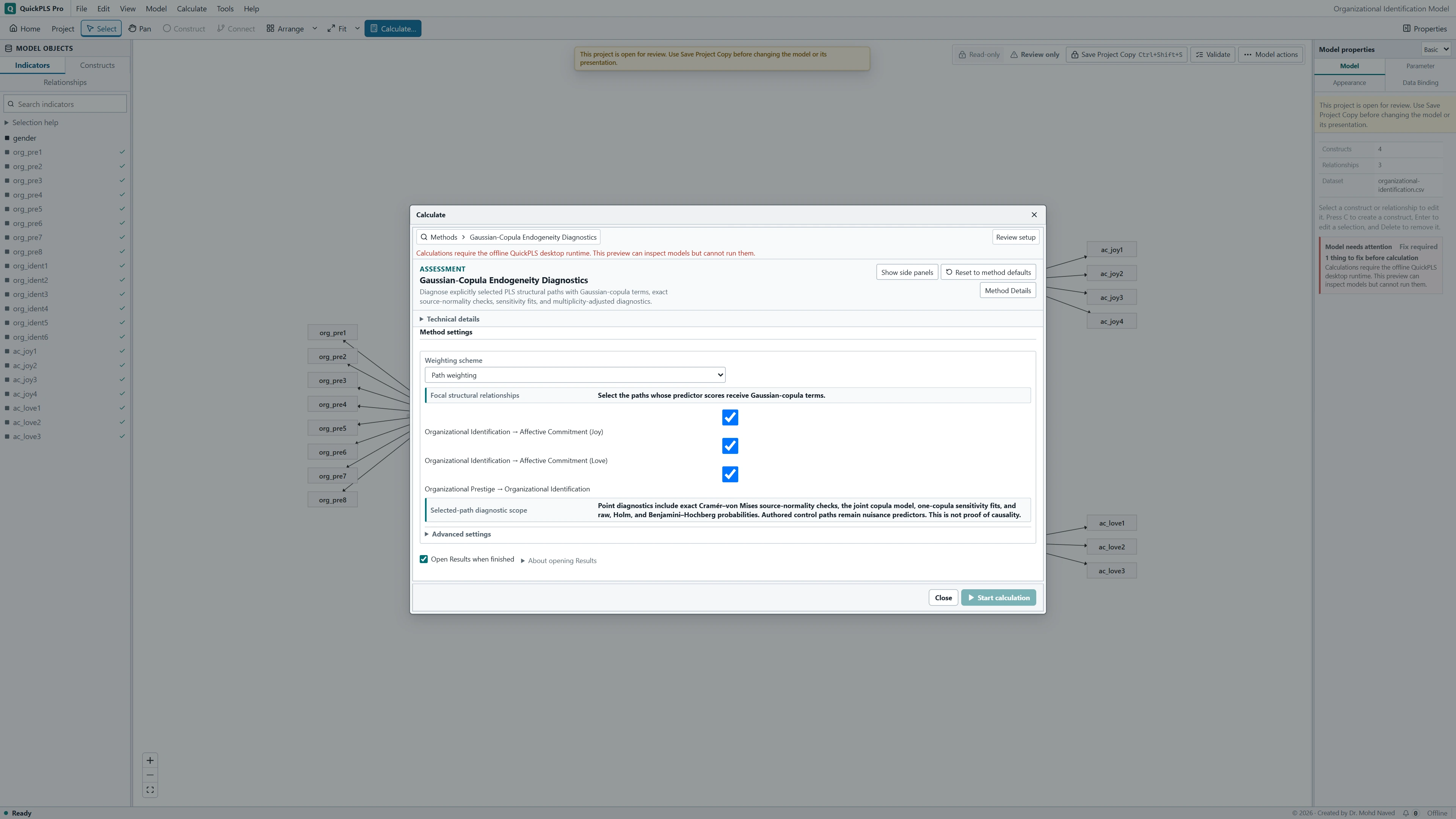
In the focal-path checklist, select the relationships whose predictors should receive copula controls. Existing control paths in the model remain included. Review the joint selection rather than assuming that each checkbox runs an unrelated model.
Calculate and read the diagnostic
Use Start calculation in the Calculate window; a dedicated diagnostic workspace labels its action Start Gaussian-copula diagnostic. Keep Open Results when finished selected. Read the predictor-normality checks, adjusted coefficients and probability adjustments together.
Read the distribution check before the probability
Find Gaussian-copula diagnostics in the completed result. Begin with the predictor's Cramér–von Mises normality check, which assesses whether its distribution is consistent with a normal shape. Then inspect the original and adjusted paths, the copula terms and any collinearity or identification warnings.
The diagnostic fits the selected copulas jointly and also reports one-copula-at-a-time sensitivity fits while retaining the model's existing controls. Read the raw p values and the Holm or Benjamini–Hochberg adjustments with their stated comparison families. These p values assess the stated null hypotheses; they are not probabilities that endogeneity is present or bootstrap confidence intervals.
On a small screen, swipe the table sideways to see every column.
| Output | How to read it | What to check |
|---|---|---|
| Source-normality checks | Checks of the selected predictor's distribution relevant to this method. | If a method requirement is not met, explain the limitation before interpreting an adjusted coefficient. |
| Copula and adjusted coefficients | Coefficients from equations that include the declared copula terms. | Read joint and sensitivity fits together. |
| Multiplicity-adjusted diagnostics | Results adjusted to account for the chosen set of tests. | Do not report only the most favourable unadjusted probability. |

Use all the evidence behind an adjusted path
Ask three questions: does the distribution support the diagnostic, does the adjusted coefficient differ meaningfully, and how uncertain is that conclusion? A small probability for a copula term does not, by itself, establish either the size of the original bias or a causal effect.
Illustrative example, not a software benchmark
A path changes after adjustment, but its predictor does not meet the relevant distribution requirement. That changed coefficient cannot be presented as a reliable correction under this method. Report the unmet assumption and reconsider the design or another justified way to address the suspected bias.
Practice: question the Quality → Satisfaction path
Download research-workshop.csv and build reflective Quality, Trust, Satisfaction and Loyalty blocks from their indicators. Use Quality → Satisfaction, Trust → Satisfaction and Satisfaction → Loyalty. Keep the Trust path in the model while examining Quality.
Before opening the diagnostic, state the concern about Quality → Satisfaction. For example, an unmeasured preference could plausibly affect both reported Quality and Satisfaction. This is a teaching hypothesis, not a claim that the synthetic file has that causal problem.
The numerical examples below are hypothetical. Use them to learn how to read the output; record the actual values from your saved practice result separately.
Run the planned focal-path check
Save and inspect the base model
Verify item coding, measurement quality and the three structural paths. Save the model so the diagnostic refers to a known specification.
What you should see: The original equation and questioned predictor are defined.
How to read it: State the reason for the endogeneity concern before running a diagnostic.
Select the diagnostic
Open Calculate… → Gaussian-Copula Endogeneity Diagnostics. In the focal structural-relationship checklist, select Quality → Satisfaction. Keep Trust → Satisfaction as an authored model path; it remains an adjustment predictor without needing to be selected as another focal concern.
What you should see: The copula calculation identifies the intended predictor and outcome.
How to read it: Confirm any controls retained in the equation.

Gaussian-Copula Endogeneity Diagnostics settings in QuickPLS. Select your own dataset and model, then use the choices described in the steps. Review the selected scope
Check which paths receive copula controls. If you select several focal paths, the joint diagnostic includes their controls together and also supplies one-copula-at-a-time sensitivity fits. Do not describe those as separate prespecified studies.
What you should see: The distribution and adjustment choices match the selected variables.
How to read it: Investigate unmet assumptions before interpretation.
Run and open the result
Start the calculation with Open Results when finished selected. If using the dedicated workspace, its run button is Start Gaussian-copula diagnostic. This point diagnostic does not ask you to choose bootstrap draws.
What you should see: The result distinguishes focal coefficients and copula terms.
How to read it: Compare with the same original equation and cases.
Read the checks in order
Open Gaussian-copula diagnostics. Review the source-normality and identification checks, the original and adjusted paths, then the copula-term probabilities. Compare the joint fit with the single-copula sensitivity fits and identify the family used for each adjustment.
What you should see: The comparison retains diagnostics and uncertainty.
How to read it: A favourable coefficient does not establish that all endogeneity has been removed.
Explain a coefficient change without overstating it
Suppose the original Quality → Satisfaction estimate is 0.35 and the adjusted estimate is 0.22. A copula term has a raw probability of 0.03 and a Holm-adjusted probability of 0.08. The adjustment changed the fitted relationship, but the inferential conclusion depends on the planned comparison family and rule. Report both values rather than selecting the smaller one.
The adjusted 0.22 is not automatically the true causal effect. Its interpretation still depends on the predictor distribution, the other model paths and the adjustment assumptions.
Now suppose a copula probability is 0.40 while the predictor is nearly normal and the copula control is highly collinear with it. The useful conclusion is that this diagnostic offers limited evidence in that setting. It is not proof that endogeneity is absent. All numbers here are hypothetical.
When the diagnostic is weak or surprising
Check the source score distribution and the model's focal-path selection before changing the analysis. If identification is weak, explain why the diagnostic cannot settle the question. The table suggests checks that preserve the research question rather than chasing a lower probability.
On a small screen, swipe the table sideways to see every column.
| Symptom | Check | Reasonable action |
|---|---|---|
| No focal relationship is selectable | Check that the saved model has eligible structural paths. | Select an actual structural relationship. Do not treat a control or measurement arrow as an equivalent focal path. |
| The source-normality result is weak or ambiguous | Inspect both the formal check and the predictor distribution. | Report limited diagnostic applicability. Do not transform a variable solely to manufacture nonnormality and a desired answer. |
| Adjusted coefficients have very large standard errors | Check overlap between predictors and their copula transforms and inspect joint sensitivity fits. | Describe instability and reconsider the identification strategy. A larger sample or a better design may be needed; a different significance cutoff is not a remedy. |
| Raw and adjusted probabilities lead to different decisions | Check the tested family and the selected multiplicity convention. | Use the predeclared rule and report both values. Do not drop other focal paths after seeing the correction. |
| A nonsignificant copula is being treated as proof of no endogeneity | Check assumptions, precision and other sources of bias. | State what the diagnostic did and did not detect. Use evidence from the study design before concluding that predictors are unrelated to the structural error. |
Keep the planned controls and compare the stated fits
Compare the joint selected-copula fit with the one-copula-at-a-time fits. If the conclusions differ, examine overlap among predictors and controls. Explain that dependence rather than presenting only the fit with the most favorable result.
Do not transform a predictor just to manufacture nonnormality, remove a justified control to lower a probability, or expand the focal-path list until a result appears. Any revised model needs a substantive reason and a clear label as a follow-up analysis.
If the concern remains unresolved, consider stronger temporal ordering, improved measurement, relevant omitted variables or a defensible instrumental-variable design. A diagnostic can guide that decision without claiming to repair the study by itself.
Write a cautious, useful diagnostic conclusion
Methods example: We investigated the prespecified Quality → Satisfaction path using a Gaussian-copula diagnostic. Trust remained in the Satisfaction equation. We examined predictor normality, copula-control identification, the joint fit and single-copula sensitivity fits, and reported probabilities with their stated multiplicity adjustment.
Results example: In the hypothetical illustration, the path changed from 0.35 to 0.22. The copula term's raw probability was 0.03 and its Holm-adjusted probability was 0.08. We interpreted the change with the distributional diagnostics and did not treat it as proof of causality or of a known amount of removed bias. Replace the example numbers with your actual output.
| Field | Report |
|---|---|
| Concern | The suspected cause of endogeneity and the path examined. |
| Assumptions | Predictor distribution and assumptions needed to distinguish the copula term's contribution. |
| Specifications | Original, joint copula and one-copula sensitivity equations. |
| Results | Coefficients, uncertainty, raw and adjusted probabilities. |
| Conclusion | What changed, what remains uncertain and any design response. |
Before drawing a conclusion
- Explain why the selected predictor may be related to the unexplained part of its outcome equation.
- Identify the source-normality result and any identification or collinearity warning.
- Compare the original and adjusted path with the planned joint and sensitivity fits.
- Name the raw or adjusted probability used and its comparison family.
- Explain why a weak copula result does not establish exogeneity and what further design evidence would help.
Report the concern and the diagnostic together
- Name the focal paths and explain why their predictors may be endogenous.
- Describe score-normality checks and any collinearity or identification problems.
- Report the original and adjusted paths, joint and single-copula sensitivity fits, and the relevant raw and adjusted probabilities.
- Keep the model's control paths and the tested comparison families explicit, and describe the result as a diagnostic rather than causal proof.
Do not read a nonsignificant control as proof of no problem
A weak or nonsignificant copula term can reflect limited information, including a predictor distribution that makes the adjustment hard to identify. It does not prove that the predictor is unrelated to the equation's error.
The diagnostic also does not resolve every omitted variable or reverse-causality concern. Use the findings alongside theory, measurement and study design. Instrumental-variable methods, if considered, require their own relevance and exclusion justification.