 QuickPLS
What the method does
Consistent partial least squares (PLSc) starts with PLS construct scores and uses estimated reliability to correct their correlations for attenuation. It then estimates relationships between the common factors represented by the reflective blocks. The correction changes the target of estimation, so PLSc should follow a factor interpretation of the indicators rather than a preference for larger path coefficients.
Corrected correlation: rᶜⱼₖ = rⱼₖ / √(ρⱼρₖ).
Here rⱼₖ is the correlation between two construct scores and ρⱼ and ρₖ are their estimated score reliabilities. This expression explains the attenuation correction. The corrected matrix must still be admissible before its structural estimates can be interpreted.
Data and analysis in QuickPLS
Use numeric case-level indicators in eligible reflective blocks with at least two indicators per block. Specify the same data preparation and model when comparing PLSc with ordinary PLS.
In QuickPLS, choose Consistent PLS for your own model. Inspect PLSc correction reliability and the original and corrected construct correlations before reading the paths. Use PLSc Consistent Bootstrapping for their uncertainty.
Follow a worked example
The following example shows the data, settings and decisions for one analysis. Use the linked practice files to follow it. For your own study, keep the procedure and choose the variables, model and settings that fit your research question.
Download research-workshop.csv to begin. It contains 360 rows and 31 columns. The example below identifies the variables to use, their roles and any rows to exclude; not every column is an analysis variable.
Choose PLSc when the items measure an underlying factor
Suppose several survey questions are intended to reflect the same underlying idea, such as Trust. You treat the idea as the reason the answers are related. That is a reflective common-factor model. It differs from a composite, where the measurements are ingredients used to define a score.
Consistent PLS, abbreviated PLSc, starts from PLS estimates and applies a correction for eligible reflective factor models. The correction uses estimated reliability, a measure of how consistently the indicators represent the factor. Choose it because that measurement interpretation fits your study, rather than because it produces a larger coefficient.
The correction must also produce valid correlations. A correlation matrix is a table of relationships among constructs. If the corrected values cannot form a valid matrix, pause the interpretation and investigate the indicators, coding and construct definitions. The sections below show both a valid arithmetic example and an invalid one.
Practise with four reflective constructs
Use research-workshop.csv to study Quality, Trust, Satisfaction and Loyalty. Give each construct its three matching indicators and draw Quality → Satisfaction, Trust → Satisfaction and Satisfaction → Loyalty. To compare with ordinary PLS, run that method separately on this same workshop file and model. The first PLS lesson uses a different, 240-case file, so its answer values are not answers for this workshop.
Assign quality_1, quality_2 and quality_3 to Quality; trust_1, trust_2 and trust_3 to Trust; satisfaction_1, satisfaction_2 and satisfaction_3 to Satisfaction; and loyalty_1, loyalty_2 and loyalty_3 to Loyalty.
For this exercise, suppose each group of indicators reflects a common factor. A factor is the underlying idea the items are intended to measure. Ordinary PLS component correlations are not automatically estimates of relationships between error-free factors; PLSc applies its reliability-based correction under the eligible reflective assumptions.
The continuous scores are invented for teaching. Their names do not establish that a factor model is correct. Explain why each block is reflective, check the direction of its indicators and consider whether the constructs have distinct meanings.
This is a comparison of estimators for a stated model. The correction does not remove omitted influences from the structural relationships or turn a poorly defined scale into a sound measure.
Check that the measurement model suits the correction
Use reflective blocks with at least two indicators per block. An indicator is a measured column; a block is the group assigned to one construct. Confirm that all items in a block have a defensible relationship to the same underlying idea.
Check the item direction and reliability before calculation. The structural paths must have no feedback loop, meaning a chain of arrows must not lead back to its starting construct. Keep a copy of the model and data you will compare with ordinary PLS.
Run Consistent PLS and inspect the correction first
For this exercise, select the saved four-construct model bound to research-workshop.csv. The ordinary PLS comparison must use that same file and model; the earlier 240-case customer answer table is not its reference.
Open the method for your model
With the intended model open, click Calculate…. Type Consistent PLS into Find a method and select that row. Check that the intended indicators are assigned to each construct.
Set the visible point-estimation controls
For the first workshop run, choose Weighting scheme → Path weighting, Result data → Standardized, and Missing data → Casewise deletion. Factor weighting is an alternative choice for a separately recorded comparison; PCA weighting is unavailable here. Expand Advanced settings to inspect Maximum iterations and Stop criterion. These are editable PLSc controls.
Start and inspect the correction
Review Readiness, leave Open Results when finished selected, and click Start calculation. In Results, open Reliability and validity → PLSc correction reliability. Then open Discriminant validity → PLSc construct correlations; Original and Corrected are columns in this one table. Inspect them before interpreting corrected paths, loadings or R-square.
Calculate the workshop model and compare the correction
Build and check the reflective model
In Indicators, select each construct's three columns with Ctrl and click Create construct. Select the new construct, open Properties → Model, enter its Name and press Enter. Under Parameter → Measurement model, choose Reflective. Choose Connect and drag from each source construct's body to its destination to make the three stated paths. Return to Select. Keep generated interactions and higher-order constructs out of this first exercise.
What you should see: Four reflective blocks and the three stated paths are visible.
How to read it: Correct assignments or arrow directions before comparing estimators.
Open Consistent PLS
Click Calculate… and use Find a method to select Consistent PLS for the same dataset and model as the ordinary PLS comparison.
What you should see: Consistent PLS is selected for the same model and dataset.
How to read it: Changing either would confound the estimator comparison.
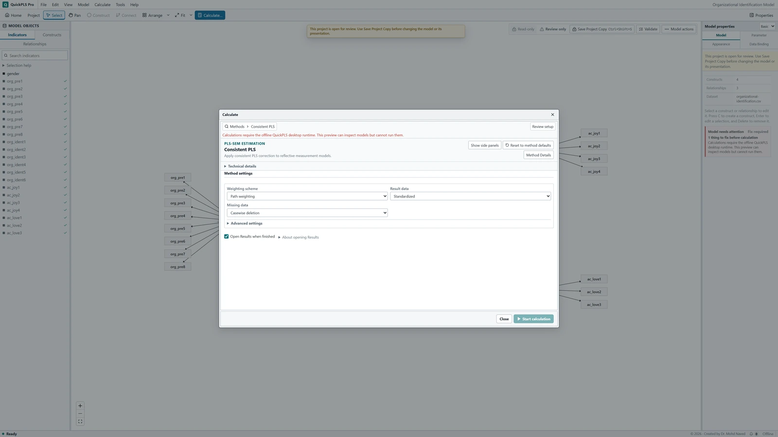
Consistent PLS settings in QuickPLS. Select your own dataset and model, then use the choices described in the steps. Choose the first-run settings
Choose Path weighting under Weighting scheme, Standardized under Result data, and Casewise deletion under Missing data. Expand Advanced settings to inspect Maximum iterations and Stop criterion, and record their displayed values. Path and factor weighting are supported alternatives; PCA weighting is not a PLSc option. Review Readiness, then click Start calculation.
What you should see: The completed result identifies the requested PLSc settings.
How to read it: Check convergence before reading the correction.
Review the reliability correction
In Results, expand Reliability and validity and choose PLSc correction reliability. Read rho_A for each eligible block and its warnings. If a reliability value is materially outside its valid range, investigate the measurement before using the corrected model.
What you should see: PLSc correction reliability lists a value for each eligible block.
How to read it: Investigate inadmissible values before using corrected paths.
Compare Original with Corrected
Expand Discriminant validity and open PLSc construct correlations. Compare the Original and Corrected columns for each pair. Check that the correction produces valid estimates, then use Search result outputs to locate Outer loadings, Direct effects and R-square in this PLSc run. Keep the corrected quantities together when reporting the analysis.
What you should see: Original and Corrected correlations appear for the same construct pairs.
How to read it: A correction outside the admissible range requires investigation, not interpretation as a strong relationship.
Add matching confidence intervals
Return to Calculate… and select PLSc Consistent Bootstrapping. Match Weighting scheme and Result data to the point run. Review Bootstrap samples, Confidence level (%), Hypothesis test and Confidence intervals. Percentile and BCa is the standard interval choice; Also compute studentized intervals reveals Inner samples per bootstrap sample. Seed is inside Advanced settings, alongside Maximum iterations and Stop criterion. Read the selected setup before starting; ordinary PLS intervals are not substitutes for these refits.
What you should see: The matching consistent bootstrap provides uncertainty for corrected estimates.
How to read it: Keep its usable draws and interval method with the result.

Read the corrected correlations before drawing a conclusion
Open Discriminant validity → PLSc construct correlations. Read each construct pair across the Original and Corrected columns. These columns show the relationships before and after the correction; they are not two separate result screens. Check that the corrected values form a valid correlation matrix before explaining the model.
Use Search result outputs to find Outer loadings, Direct effects and R-square in the selected PLSc result. A loading relates an indicator to its construct; a direct effect describes a relationship between constructs. R-square describes the variation explained for a fitted outcome. Keep these corrected results together and clear the search afterwards.
Open Reliability and validity → PLSc correction reliability to read rho_A for each reflective block, then review Diagnostics and warnings. Reliability is part of the correction, so an unstable reliability estimate can make the corrected result unstable. A larger number of bootstrap draws cannot make an invalid original correction valid.
On a small screen, swipe the table sideways to see every column.
| Output | How to read it | What to check |
|---|---|---|
| Corrected correlations | Relationships after the consistent correction. | Check whether the corrected correlations form a valid solution before interpreting paths. |
| Corrected paths and loadings | Estimates for the stated reflective factor model. | Compare like quantities, not corrected paths with uncorrected weights. |
| rho_A and warnings | Reliability estimates and checks required for the consistent correction. | Unstable correction is not fixed by a larger bootstrap count. |

Understand why PLS and PLSc can give different paths
How to compare two estimators
Two researchers can analyse the same indicators with PLS and PLSc and obtain different path estimates. They asked for different calculations with different measurement interpretations. Match the estimator, data and settings before judging agreement between programs. To describe uncertainty around a corrected estimate, use the matching PLSc bootstrap rather than an ordinary PLS interval. This explains the comparison; it is not a new numerical benchmark.
Explain why you used the consistent correction
- Describe why the indicators are reflective measures of a common factor.
- Name Consistent PLS, the weighting choice and the measurement requirements used.
- Report correction warnings and use the corresponding PLSc calculation for confidence intervals and tests.
Investigate an invalid correction instead of hiding it
PLSc's reflective correction is not a correction for formative composites, whose indicators define the composite. The measurement interpretation determines whether the procedure fits the question.
If a corrected correlation is invalid, check coding, reliability and overlap between constructs. Do not cap it at an acceptable-looking value. Switching to ordinary PLS changes the analysis; it should be described as a separate choice with its own reason.
See what the reliability correction does to a correlation
Take an illustrative original correlation of 0.50 and reliabilities of 0.81 for both constructs. Divide the correlation by the square root of 0.81 × 0.81. The corrected value is approximately 0.6173. The factor interpretation allows for the weakening of an observed relationship through imperfect measurement.
This example concerns an off-diagonal entry, a correlation between two different constructs. The original value and the reliability estimates are inputs to the correction; the method does not simply add a fixed amount to every path.
Now try an original correlation of 0.90 with reliabilities of 0.64 and 0.64. The corrected value is 1.40625. A valid correlation cannot exceed 1, so this correction is inadmissible. Cutting it back to 1 would conceal the problem.
If you see such a problem, inspect coding, overlap between constructs and the factor assumptions. Three indicators give more measurement information than two, but a particular indicator count cannot guarantee a valid correction.
On a small screen, swipe the table sideways to see every column.
| Output | Hypothetical example or task | Reading |
|---|---|---|
| rho_A | 0.81 for both blocks in the arithmetic example | Reliability enters the correction; inspect warnings and admissibility. |
| Original correlations | 0.50 | The correlation between component scores before correction. |
| Corrected correlations | 0.6173 after the example correction | The estimated correlation between factors under the reflective assumptions. |
| Corrected paths and R-square | Inspect the full set of corrected model estimates. | Paths depend on the whole predictor correlation structure. |
| Corrected loadings | Read with the block and scale | They are not ordinary PLS loadings merely renamed. |
| Correction warnings | Example corrected correlation 1.40625 is invalid | Do not cap the value at 1 and continue reporting. |
Check the inputs when a correction cannot be interpreted
Start with the original result and the exact warning. If Readiness blocks the calculation, return to the model and check that each intended block is Reflective and has enough assigned indicators. In Calculate, check Weighting scheme; PCA weighting is not available for PLSc. A rejected calculation is different from an invalid correction in a completed result.
In Results, use PLSc correction reliability and the Original and Corrected columns of PLSc construct correlations to locate the problem. Check indicator assignment, reverse coding and overlap between constructs. If the original correction fails, report that outcome. If only some bootstrap refits fail, report their number and reasons alongside any available intervals.
On a small screen, swipe the table sideways to see every column.
| Symptom | Check | Reasonable action |
|---|---|---|
| rho_A is nonpositive or materially above one | Coding, block specification and finite-sample behaviour | Investigate the measurement model; report the failed correction. |
| A corrected correlation exceeds the valid range | Reliabilities and overlap between constructs | Reconsider the factor distinction; do not clip the correlation. |
| PLSc and PLS paths differ | Estimator target, correlations and matched settings | Explain the factor-versus-component interpretation rather than declaring one universally superior. |
| The chosen weighting option is unavailable | Path or factor versus PCA weighting | Use a supported PLSc option only if it fits the intended analysis. |
| Bootstrap intervals do not match the point model | Whether consistent correction was applied during refits | Use matching PLSc inference and report failed corrections among resamples. |
Compare PLS and PLSc without changing the question
Hold the sample, indicators, coding and paths fixed. First compare the original and corrected correlations, then inspect the path estimates. When an outcome has several predictors, changing several correlations can change a path in a way that is more complicated than increasing it by one multiplier.
Ask whether both measurement interpretations are defensible for your study. A designed composite may be appropriate because its indicators define it. A common-factor correction should follow a factor interpretation, not a search for the estimator with the preferred probability or coefficient.
If a measurement revision is justified, save it separately and explain what changed. Repeatedly removing indicators until a correction becomes valid is an exploratory search. Keep a record of that search and avoid presenting its final model as though it was the only model considered.
Report the correction and its uncertainty together
For this workshop, a Methods description could read: We fitted the reflective four-construct model using Consistent PLS and the recorded path-weighting and preprocessing settings. We inspected rho_A and the corrected construct correlations before interpreting corrected paths, loadings and explained variance. We assessed uncertainty using the corresponding consistent bootstrap.
For the arithmetic example, a Results explanation could read: An original construct correlation of 0.50 with reliabilities of 0.81 was corrected to approximately 0.6173. This demonstrates the operation and is not a fitted correlation from the workshop data.
In your research report, replace that illustration with the actual corrected estimates, matching intervals and any correction failures. If a path is weak or uncertain, explain its size and uncertainty instead of changing estimators solely to obtain a more favourable result.
| Item | Report |
|---|---|
| Measurement interpretation | Why the blocks are reflective common-factor measures |
| Estimator and settings | Consistent PLS; path or factor weighting; preparation |
| Correction assessment | rho_A, original and corrected correlations, warnings |
| Model estimates | Corrected loadings, paths and R-square |
| Inference | Matching consistent bootstrap, interval method and usable counts |
| Comparison | Any ordinary PLS analysis identified separately |
Check that you can explain the correction
- Recalculate the illustrative corrected correlation of 0.6173.
- Explain why 1.40625 cannot be accepted as a correlation.
- Locate the Original and Corrected columns in PLSc construct correlations.
- Confirm that the paths and intervals you report come from the same estimator.
- Explain why the indicators in your study should be treated as reflective factor measures.