 QuickPLS
What the method does
Structural path randomization builds a reference distribution by breaking a specified relationship while retaining the structure required by the chosen test. This workflow conditions on fixed PLS scores. It therefore answers a different question from a case bootstrap that refits the measurement and structural model in every sample.
Randomization tail probability: p = (E + 1) / (B + 1).
E counts reference statistics at least as extreme as the observed statistic and B is the number of usable randomizations, under the selected tail rule. The statistic and randomization scheme define the null hypothesis; state them with the result.
Data and analysis in QuickPLS
Use an eligible fitted PLS model and specify the paths or equations to test. Check that the exchangeability assumptions suit the analysed cases.
QuickPLS provides the structural-path randomization settings and test results. Keep the fixed-score interpretation and the requested and usable reference counts with the reported probability.
Follow a worked example
The following example shows the data, settings and decisions for one analysis. Use the linked practice files to follow it. For your own study, keep the procedure and choose the variables, model and settings that fit your research question.
Download research-workshop.csv to begin. It contains 360 rows and 31 columns. The example below identifies the variables to use, their roles and any rows to exclude; not every column is an analysis variable.
Ask how unusual the path coefficient is with these scores
Structural Path Randomization tests every direct path in the converged PLS model. Before calculating, identify the paths that answer your planned hypotheses. For each path, the procedure holds the original construct scores fixed and uses the Freedman-Lane residual shuffle within its structural equation. It therefore asks a narrower question than an analysis that re-estimates the measurement model from indicators each time.
For each path, the procedure first fits the outcome without that path, keeping the other predictors in the equation. This is the reduced equation used in the shuffle. Its p-value describes how unusual the observed coefficient is under the stated zero-path hypothesis and randomization assumptions. Each value is unadjusted for testing several paths. Decide how you will interpret the full set of planned hypotheses rather than selecting only a small p-value after seeing the table.
Record the model and planned path hypotheses
Fit and inspect the ordinary PLS model, including its construct scores and predictor relationships. Record your planned path hypotheses and the other predictors in each equation before randomization. The procedure calculates all direct paths; there is no separate path-selection control for this method.
Run the structural residual randomization
Open the intended model
Open Calculate and choose Structural Path Randomization. Keep the model and data preparation that produced the intended PLS score solution.
Set the repetition plan
Set Permutations and Seed. The procedure tests the direct paths in the model. Identify your planned focal paths in the result rather than looking for a path-selection setting.
Read the path rows with their assumptions
Calculate and inspect Original, Exceedances, Permutations and Raw two-sided p for each planned path. The probabilities are conditional on the fixed scores and unadjusted for multiple testing.
Read the observed coefficient and its randomization count
The fixed construct scores supply the observations for the structural equations. Original is the observed path coefficient; Exceedances counts randomized coefficients at least as extreme under the two-sided comparison. Read Raw two-sided p with the stated permutation count. This test does not re-estimate all measurement uncertainty and does not shuffle group labels.
On a small screen, swipe the table sideways to see every column.
| Output | How to read it | What to check |
|---|---|---|
| Original construct scores held fixed | The original scoring solution used for the randomization. | Measurement uncertainty is not fully re-estimated here. |
| Randomized path statistic | The coefficients calculated after shuffling residuals, used to assess the selected path. | Do not call this a cross-group permutation. |
| Pathwise probability | Unadjusted evidence for the individual selected path. | Account for the full set of hypotheses when reporting many path tests. |

State which values were randomized and which stayed fixed
Illustrative example, not a software benchmark
The word permutation can describe different analyses. Randomizing structural residuals while keeping scores fixed is not equivalent to reassigning group labels and refitting PLSc. State what was randomized, what remained fixed and which hypothesis the reference calculation represents.
Test Quality while retaining Trust in the equation
In the service model, Quality and Trust both predict Satisfaction. To test the Quality path, the procedure first fits Satisfaction without Quality but with Trust. It shuffles the residuals, the part left unexplained by that reduced equation, and adds them back to the reduced fitted values. The resulting synthetic outcome is then fitted with the full equation, including Quality.
Build the four reflective constructs from the research workshop file, with Quality → Satisfaction, Trust → Satisfaction and Satisfaction → Loyalty. Fit ordinary PLS first. The estimated construct scores remain fixed during randomization. The resulting test is conditional on those scores and does not include all uncertainty from estimating the measurement model.
Follow the focal path through the residual shuffle
Inspect the score model and predictors
Check coding, convergence and the structural equation. For Quality → Satisfaction, Quality is the focal predictor and Trust is the other predictor retained in the reduced equation. The reduced equation also has an intercept. Use the complete-data teaching model without weights or extra extensions.
What you should see: The fixed-score equation contains the intended predictors.
How to read it: This test conditions on those scores.
Set the randomization plan
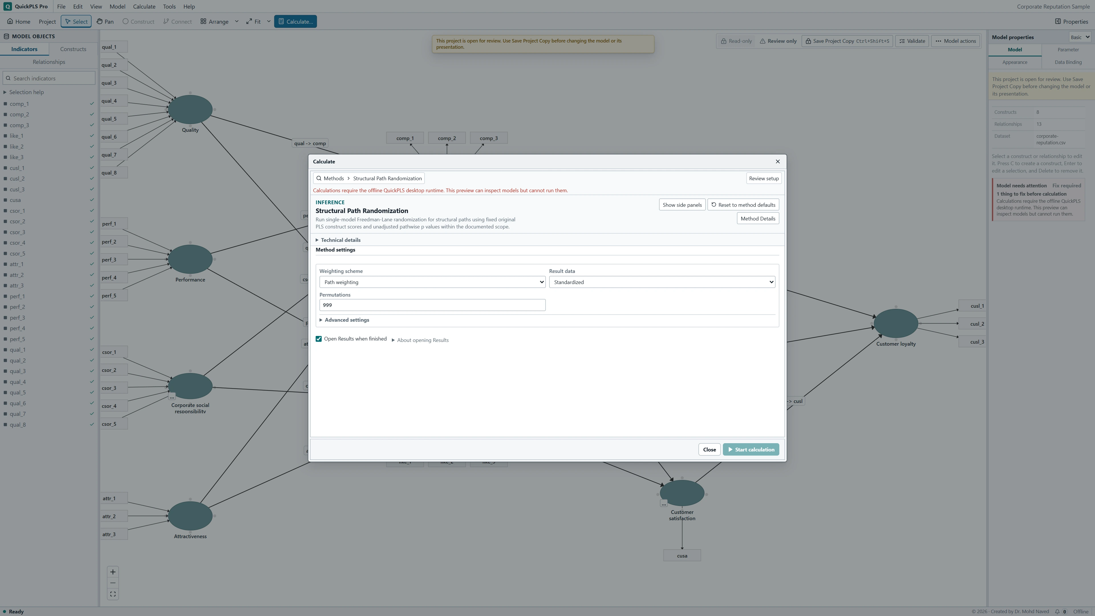
Open Calculate and choose Structural Path Randomization. Set Permutations to 999 and Seed to 20261105 for this exercise. The supported range is 99 to 10000. Record the estimator and model settings behind the fixed scores. The calculation tests all direct paths; use the Quality row for the planned focal interpretation. Review Readiness and click Start calculation. In Results, use Search result outputs to open Structural path randomization.
What you should see: The selected scheme, statistic, tail rule and seed are explicit.
How to read it: Together they define the null comparison.
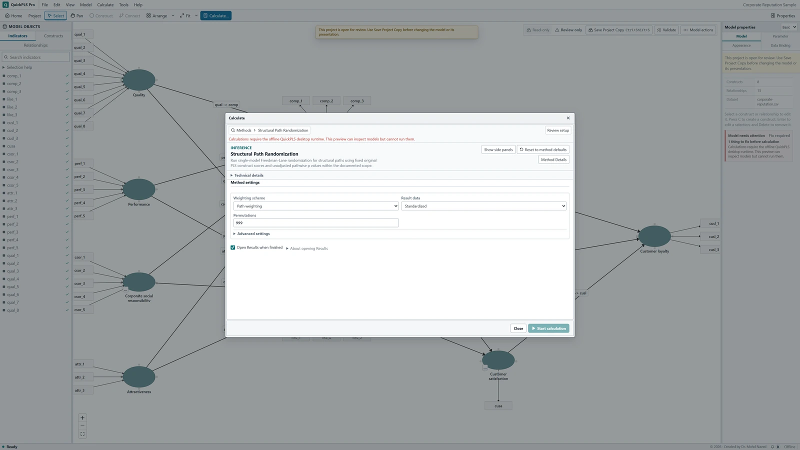
Structural Path Randomization settings in QuickPLS. Select your own dataset and model, then use the choices described in the steps. Understand what is shuffled
For the Quality path, the reduced equation predicts Satisfaction from Trust and an intercept. Its residuals are shuffled across cases and added to its fitted values. Shuffling Satisfaction directly would also remove the fitted contribution of Trust and would ask a different question.
What you should see: The shuffled quantity matches the selected randomization scheme.
How to read it: Do not interpret it as resampling whole cases and refitting the measurement model.
Understand the full-equation refits
Each randomized outcome is regressed on the full predictor set, including Quality. Its focal coefficient is compared with the observed one. The procedure uses a two-sided, unadjusted add-one probability to test a zero coefficient while retaining the original scores and the other predictors.
What you should see: The reference equations retain the intended nuisance structure.
How to read it: Compare like-for-like statistics.
Keep failures and the denominator visible
Inspect the completion status and numerical failures. A required fitting failure prevents the inferential result; the procedure does not silently drop failed randomizations and reduce the denominator. Export the path row, permutation count, seed and method description together.
What you should see: The tail count and usable reference denominator are identifiable.
How to read it: Report unavailable tests separately from large p-values.
Work through the add-one probability and its limits
Suppose the hypothetical Quality → Satisfaction score-regression coefficient is 0.25. Among 999 randomized results, 19 have an absolute focal coefficient at least as large as 0.25. The two-sided probability is (19 + 1)/(999 + 1) = 0.02. Under the procedure's assumptions, the observed association is unusual compared with what this procedure produces when the Quality coefficient is zero, while accounting for Trust.
If none of the 999 randomized coefficients is as extreme, the probability is 1/1000, or 0.001, not zero. Increasing the number of permutations can give finer numerical resolution. It does not turn a nonexperimental association into a causal effect, and it does not supply a confidence interval for the path.
Suppose Trust is strongly associated with Satisfaction and also correlated with Quality. Shuffling the raw Satisfaction score would break the Trust relationship as well. Shuffling the reduced equation's residuals preserves the fitted contribution of Trust. This explains why results from an unrelated raw-outcome shuffle need not match this calculation.
The residuals must be exchangeable under the null, meaning that their reassignment across cases is defensible. Repeated observations from one person, clustered employees or systematic differences in residual spread can violate that condition. The documented calibration covers a limited setting with normally distributed errors of constant variance. Having a randomization command does not establish validity for every pattern of errors.
Check the equation and the shuffle assumptions
On a small screen, swipe the table sideways to see every column.
| Symptom | Check | Reasonable action |
|---|---|---|
| A path has an unexpected sign | Indicator direction and correlations among structural predictors | Resolve coding errors and consider suppression before interpreting the probability. |
| The equation cannot be estimated uniquely | Redundant predictors or almost identical construct scores | Review the model specification. Do not remove a theoretically necessary predictor solely to make the test run. |
| The calculation stops after a failed fit | The reported randomization failure | Treat the result as unavailable and diagnose the equation; do not divide by only successful permutations yourself. |
| Residual spread changes across fitted values | Unequal error variance and dependence between cases | Use an inference method justified for that error structure. The current residual shuffle is not a general robust correction. |
| The probability differs from bootstrapping | Whether scores were fixed or fully re-estimated | Explain that the procedures quantify different uncertainty rather than selecting the smaller probability. |
Choose the follow-up that addresses the uncertainty
If you are concerned about omitted predictors, review the theory and compare a justified alternative equation while retaining the original. If the concern is unstable measurement, use full model resampling and measurement assessment. Repeating this fixed-score test cannot reveal all uncertainty from estimating the scores.
When interpreting several paths, state that the probabilities are unadjusted and explain the family of hypotheses. A larger permutation plan can improve numerical resolution near a boundary. Repeatedly changing seeds until a result becomes significant is not a sensitivity analysis; retain the original plan and state any planned follow-up.
Example wording for what stayed fixed and what was shuffled
Methods example: We used Structural Path Randomization with 999 permutations and seed 20261105. Construct scores from the original PLS fit remained fixed. For each focal path, the reduced equation retained the other structural predictors and an intercept; its residuals were permuted and added to its fitted values before refitting the full equation. We interpreted the two-sided add-one probabilities conditionally on these scores.
Hypothetical Results example: The Quality to Satisfaction coefficient was 0.25, and 19 of 999 randomized coefficients were at least as extreme in absolute value, giving p = 0.02. This supported a nonzero conditional score association under the randomization assumptions; it did not establish a causal effect or account for full measurement-estimation uncertainty.
| Report item | Detail to record |
|---|---|
| Score source | Original model, estimator and analysis cases |
| Focal test | Path and other predictors retained in the reduced equation |
| Randomization | Residual procedure, count, seed and completion status |
| Probability | Two-sided, add-one and unadjusted definition |
| Assumptions | Independent cases and defensible residual exchangeability |
Check the hypothesis and the calculation
- Identify the focal and retained predictor for Quality → Satisfaction.
- Explain why shuffling the raw outcome asks a different question.
- Calculate the smallest possible probability with 999 permutations.
- Distinguish fixed-score randomization from full PLS bootstrapping.
- Name a data structure that makes unrestricted residual shuffling inappropriate.
Report the score source, randomization and hypothesis family
- Identify the original scoring model and the paths selected for interpretation.
- Describe the Freedman-Lane residual procedure, Permutations and Seed.
- State that probabilities are unadjusted and explain how you handled multiple path hypotheses.
Keep the fixed-score test separate from other permutation methods
This is a structural-equation test conditional on estimated scores. It is neither a full indicator-level PLS permutation nor a cross-group test. Its pathwise probabilities are unadjusted, so reporting several tests requires an explicit interpretation of the hypothesis family.