 QuickPLS
What the method does
Prediction-oriented model selection evaluates alternative specifications for the same research task. Selection criteria can balance fit against complexity, while held-out prediction examines errors on cases excluded from fitting. The candidate set and selection rule should be stated in advance where possible; a search chosen after inspecting results remains exploratory.
BIC = −2 log L + k log n.
L is the likelihood under the criterion’s model, k the parameter count and n the sample size. Smaller BIC is preferred among comparable candidates. In a prediction-oriented implementation, retain the app’s equation and candidate definitions; BIC is not itself a held-out error.
Data and analysis in QuickPLS
Use a defined set of eligible models with comparable outcomes, data preparation and cases. State which differences between the candidate models are theoretically plausible.
QuickPLS reports candidate comparisons and outcome-specific selections. Check model requirements and conflicting criteria before choosing a model to report.
Follow a worked example
The following example shows the data, settings and decisions for one analysis. Use the linked practice files to follow it. For your own study, keep the procedure and choose the variables, model and settings that fit your research question.
Download research-workshop.csv to begin. It contains 360 rows and 31 columns. The example below identifies the variables to use, their roles and any rows to exclude; not every column is an analysis variable.
Select among three specified candidate models
Suppose you have three plausible explanations of Loyalty: Quality works through Satisfaction, Quality also has a direct relationship with Loyalty, or Quality uses only the direct route. Prediction-Oriented Model Selection compares the candidates you supply. It does not draw new models or search every possible arrow.
The method accepts 2 to 20 compatible saved PLS models. It uses BIC, the Bayesian information criterion, to balance fit against the number of estimated predictors. BIC is calculated separately for each outcome equation, meaning the part of a model predicting one construct.
All candidates use one raw dataset and the same eligible cases. If candidates need different indicators, a missing answer must not give one candidate a different test sample. An exact tie or different preferred models for different outcomes is a result to explain, rather than a reason to force a single winner.
Compare three routes from Quality to Loyalty
Download research-workshop.csv and the data guide. Use its 360 synthetic cases to build reflective Quality, Trust, Satisfaction and Loyalty constructs, each with its three matching indicators. Leave identifiers, group, weight and arithmetic-mean columns outside the measurement model. These invented scores support a software exercise, not validation of the constructs.
Save Candidate A with Quality → Satisfaction, Trust → Satisfaction and Satisfaction → Loyalty. This is the indirect route from Quality to Loyalty.
Save Candidate B with all of A’s paths plus Quality → Loyalty. It allows both the direct and indirect routes. Save Candidate C with Trust → Satisfaction, Satisfaction → Loyalty and Quality → Loyalty, removing Quality → Satisfaction. It uses the direct route for Quality.
Keep the same dataset, indicators and compatible ordinary PLS settings in all three. Record these alternatives before calculating. Their diagrams are practice explanations; the data generator does not establish which explanation is correct.
Write down the candidates and the decision rule
Save 2 to 20 compatible ordinary PLS models against one raw dataset. For each, record what assumption changes and why it belongs in the comparison. Decide how the outcome-specific rankings will guide your choice and how you will later assess prediction using separate data.
Under Choose candidate models, identify the saved A, B and C specifications by their paths as well as their names. If a model is unavailable, read the reason beside it before changing the candidate set.
Choose the three candidates and inspect every outcome
Fix the planned comparison
Record why A, B and C belong in the comparison and which outcomes matter. A later revision is possible, but adding a path after a promising result is an exploratory change and should be described that way.
What you should see: The candidate set and primary outcome are written down.
How to read it: Adding candidates after seeing results makes the search exploratory.
Tick the saved candidates
Open Calculate… → Prediction-Oriented Model Selection. Under Choose candidate models, tick A, B and C. The method accepts 2 to 20 compatible saved candidates and ranks this supplied set; it does not generate or modify the models.
What you should see: Only the intended saved models are selected.
How to read it: Confirm their names and specifications.
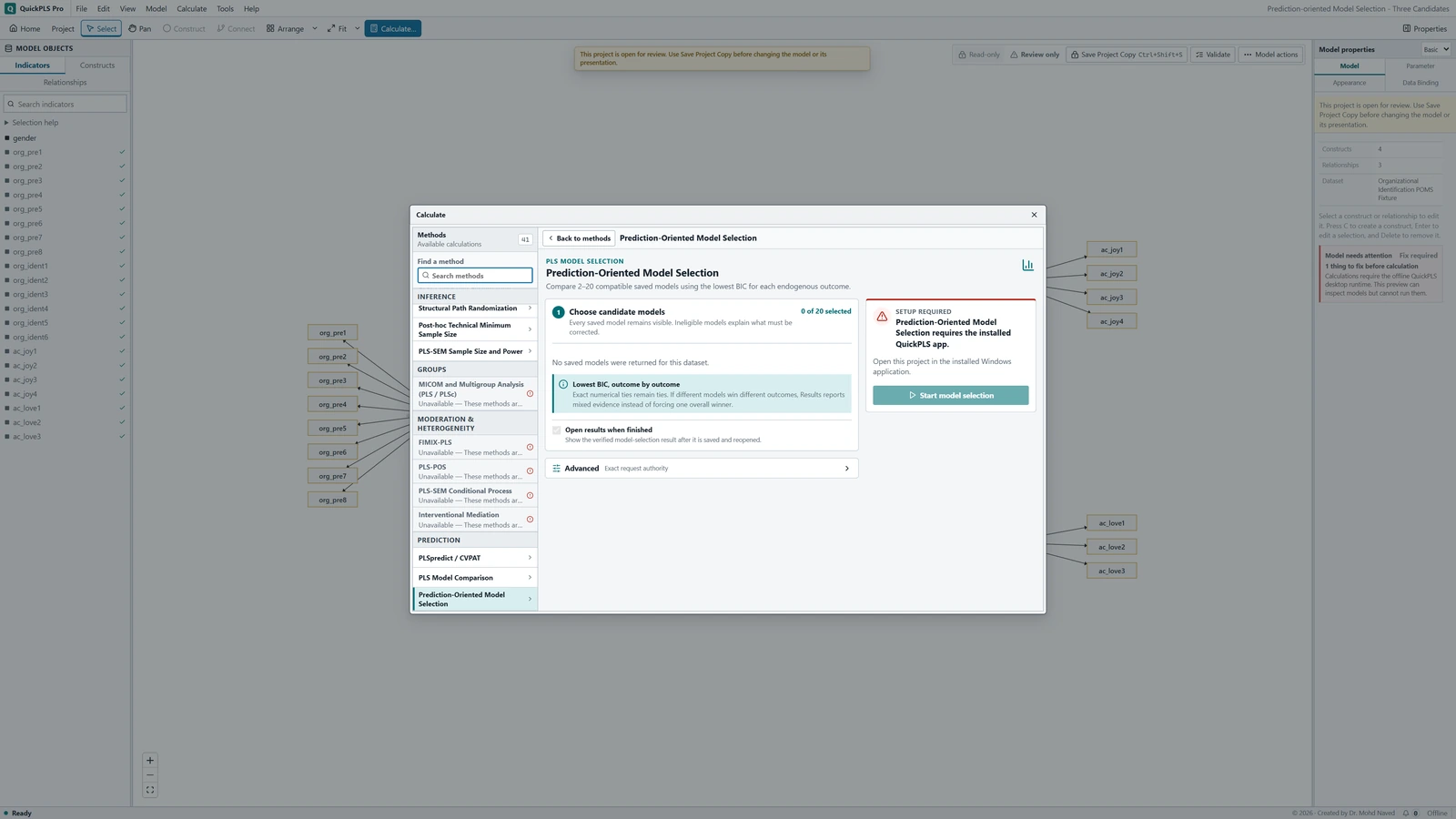
Prediction-Oriented Model Selection settings in QuickPLS. Select your own dataset and model, then use the choices described in the steps. Check the model requirements
Use one raw dataset with the ordinary PLS estimator and compatible preprocessing and missing-data policy. Keep Satisfaction and Loyalty as common outcomes. This exercise does not add PLSc, weights, higher-order constructs, fixed scores, moderation or group models.
What you should see: Each candidate meets the required model conditions.
How to read it: An ineligible candidate cannot be treated as a losing fitted model.
Review the common sample
The analysis uses rows complete across every indicator needed by every candidate. An extra indicator can therefore reduce the sample for all candidates. Check the final number of observations, rather than assuming it equals the CSV row count. This keeps model differences separate from changes in who was analysed.
What you should see: The comparison uses a common sample and target.
How to read it: Different data would confound model and sample effects.
Calculate and read the decision
Click Start model selection. Open Overview → Selection overview and Outcome decisions, then Model fit → Candidate BIC values. Read every candidate within Satisfaction and within Loyalty. Retain exact ties and different winners across outcomes; neither requires an arbitrary overall winner.
What you should see: The output identifies the selected candidate for each stated criterion or outcome.
How to read it: Interpret conflicting selections explicitly.

Equation-specific BIC and outcome decisions
Start with Outcome decisions to see which candidates have the lowest value for each outcome. Then inspect Candidate BIC values under Model fit. Lower BIC is preferred among the compatible candidates for that same equation.
Check the sample and parameter count with the value. A candidate can rank first for Loyalty and poorly for Satisfaction. The overview preserves ties and mixed evidence instead of resolving them by the order of model names.
Equal rounded display values may conceal a small stored difference. Use the full-precision ranking to decide whether a tie is exact, then apply the selection rule stated before the run. A favourable hypothesis result is not a substitute for that rule.
On a small screen, swipe the table sideways to see every column.
| Output | How to read it | What to check |
|---|---|---|
| Saved models and input data | The model specifications actually included in the ranking. | Check the data and settings as well as the model names. |
| Equation-level BIC | Read BIC separately for each relevant equation, using the reported likelihood and parameter-count definitions. | Compare values for the same outcome; lower is preferred. |
| Ties / mixed rankings | Outcomes for which candidates tie or different candidates rank first. | Keep exact ties distinct from small differences, and report mixed rankings. |
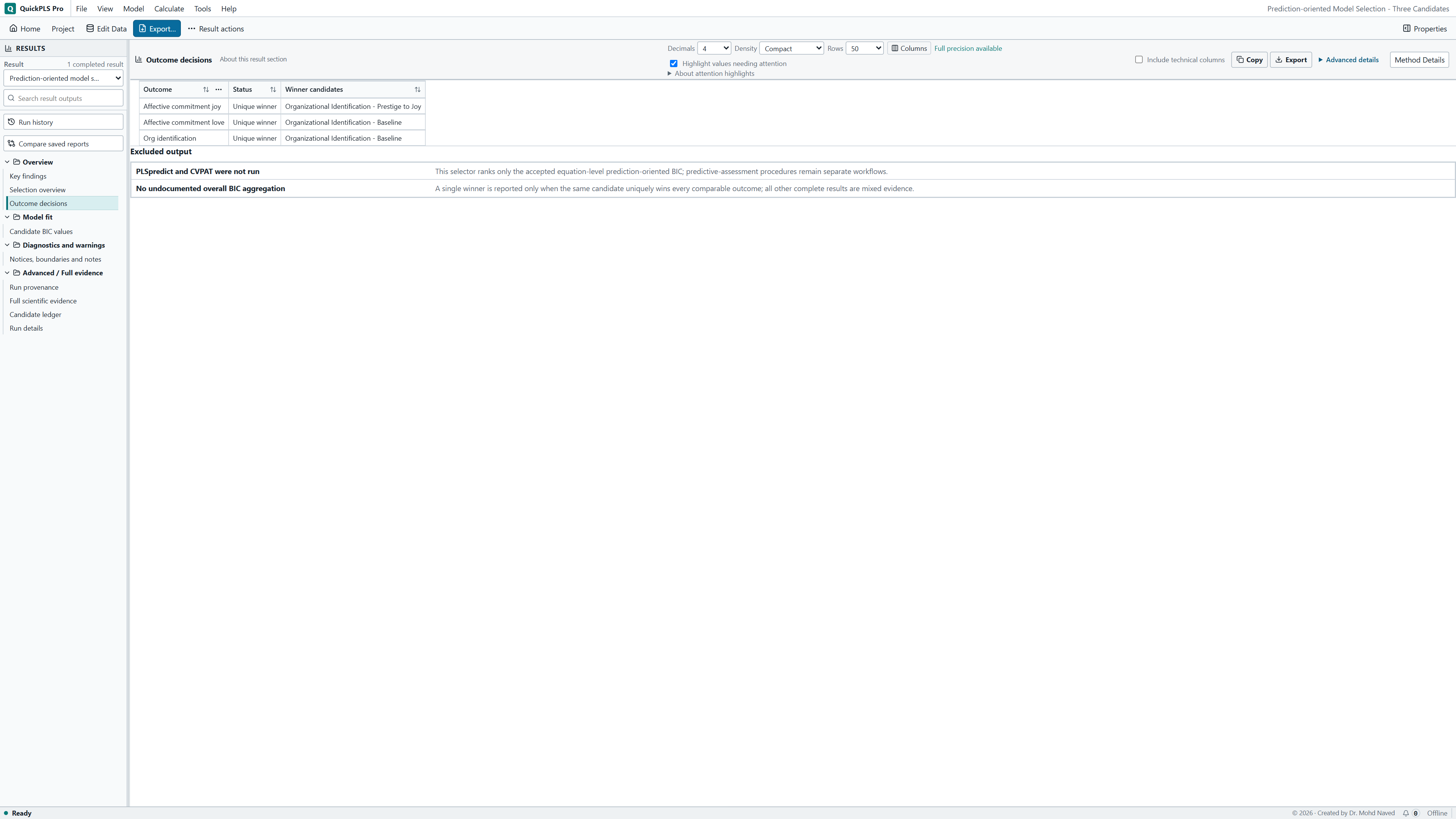
Understand a tie before choosing a winner
BIC combines the residual sum of squares, which summarises unexplained variation in an equation, with a penalty based on the number of incoming predictors plus an intercept. Smaller values are preferred for compatible candidates predicting the same outcome. This calculation uses the full common sample, not repeated cross-validation.
Take this hypothetical example, not output from the practice CSV. For Satisfaction, A has BIC 120, B has 120 and C has 128. For Loyalty, A has 104, B has 100 and C has 103. B is uniquely lowest for Loyalty but shares the minimum with A for Satisfaction.
The overall description remains mixed evidence because Satisfaction has an exact tie, even though B is never worse in this example. Display order does not break that tie.
Displayed values of 120.00 and 120.00 could also hide different stored values. Check the full-precision ranking before calling them equal. Do not add values across unrelated outcome equations to invent an overall BIC score; retain each equation’s definition and parameter count.
Eligibility checks and inconclusive comparisons
If a candidate is unavailable, begin with the reason and correction shown beside its name. If calculation fails, retain the named candidate and stage. A valid mixed ranking is different from an incomplete comparison; the table helps you choose the next step.
On a small screen, swipe the table sideways to see every column.
| Symptom | Check | Reasonable action |
|---|---|---|
| A saved model cannot be selected | Inspect estimator, dataset, outcomes and advanced model features. | Use a compatible ordinary PLS candidate or analyse the advanced model through its own method. Do not silently change its estimator. |
| The comparison rejects duplicate candidates | Check whether renamed models use the same indicators, paths and settings. | Remove the duplicate before calculating and report the distinct candidate models. |
| One candidate fails and no ranking appears | Check the named candidate and estimation stage. | Resolve its specification or report that the planned comparison could not be completed. Do not quietly drop the failed model and rank the survivors. |
| Different outcomes choose different candidates | Read each equation, sample and full-precision criterion. | Report mixed evidence and apply a previously justified outcome priority, or defer selection. A preferred hypothesis is not a selection rule. |
| BIC is unavailable for an apparently perfect fit | Check residual variance and the model parameter count. | Inspect duplicated columns or an overfitted equation. A nonpositive residual sum of squares is not handled by inventing a tiny positive value. |
Evaluate the selected model separately
After choosing a model, assess prediction with a procedure suited to its intended use. That answers a different question from this fitted-sample BIC ranking. Where the data allow it, reserve an untouched evaluation sample before choosing the model. If all observations have already informed the search, say so.
A sensitivity analysis may use a defensible alternative measurement specification. Keep the original candidate set and ranking visible, and explain the reason for the change. Removing indicators only to improve BIC does not strengthen the research rationale.
Changing the candidate set changes what winning means. A lowest value among weak candidates does not show that the selected explanation is adequate or that its predictions will be useful.
Methods and results example
After completing the exercise, a methods paragraph could say: “We specified three ordinary PLS candidates for indirect, direct-plus-indirect and direct Quality relationships with Loyalty. They used the same indicators and common complete cases. We compared prediction-oriented BIC separately for Satisfaction and Loyalty, retaining exact ties and disagreement across outcomes.” Adapt this to the saved models and run.
For the hypothetical example, write: “For Satisfaction, A and B shared BIC 120, while C had 128. For Loyalty, B had BIC 100, compared with 104 for A and 103 for C. The overall evidence was mixed because Satisfaction had an exact tie.” Explain that these are fitted-sample criteria, not independent predictive validation. Replace the invented values before reporting your own analysis.
| Report field | Required detail |
|---|---|
| Candidates | Every model considered, its paths and its substantive rationale. |
| Common sample | Dataset, all indicators required by the candidates, case exclusions and final N. |
| Criterion definition | Equation, residual sum of squares, parameter count and BIC. |
| Decision | Unique minimum, exact tie or differing outcome rankings. |
| Later assessment | How predictive performance and post-selection uncertainty were handled. |
Report the candidate set, not just the selected model
- List every candidate considered, its rationale and how the common sample was formed.
- Give the criterion values for each outcome, any exact ties and the rule used to decide what to carry forward.
- Describe the later evaluation and identify any data that were kept out of model choice.
A BIC ranking is a model-choice result
This method uses the fitted sample. It does not run cross-validation or establish how accurately the chosen model predicts new cases.
An exact tie or disagreement between outcomes may leave no single preferred model. Report that result. The best candidate in the supplied set is not automatically a satisfactory theory or a useful predictor.
Check that you can justify the selection
- Explain how the Quality paths differ between A, B and C.
- Identify the shared outcomes and the common analysis cases.
- Distinguish an exact tie from values that only look equal after rounding.
- Explain why this BIC procedure does not itself perform cross-validation.
- Write a mixed-evidence conclusion without inventing an overall winner.
Optional methods and settings
Command and output reference
Open model selection
Click Calculate… and find Prediction-Oriented Model Selection in Find a method. Continue to setup if that button is shown. Under Choose candidate models, tick the checkbox for each saved candidate.
Check eligibility and the intended sample
Read the reason and correction beside any unavailable candidate. Confirm the common dataset, outcomes and compatible settings. The analysis forms complete cases across the indicators needed by all selected candidates; inspect the final case count in the result.
Run and open the rankings
Keep Open results when finished selected and click Start model selection. In Results, open Overview → Selection overview and Outcome decisions. Open Model fit → Candidate BIC values for each candidate’s equation-specific values. Use Search result outputs if needed.
Interpreting disagreement across outcomes
The example below explains why choosing the model after seeing which hypothesis becomes significant changes the nature of the decision. Keep the outcome rankings visible, even if that leaves the choice unresolved.
Illustrative example, not a software benchmark
Suppose one candidate ranks first for one outcome and a different candidate ranks first for another. Report both rankings. Choosing afterwards according to which model makes your preferred hypothesis significant is exploratory selection, even if the original candidate models were theoretically motivated.