 QuickPLS
What the method does
Consistent permutation compares an observed PLSc group difference with differences generated after reassigning group labels under the null hypothesis. The PLSc correction belongs to each permuted fit. Measurement comparability, exchangeability and valid corrected solutions are needed for the comparison to be meaningful.
Observed contrast: Δβ = β₁ − β₂. Compare |Δβ| with the corresponding permuted contrasts.
The absolute value describes a two-sided contrast; use the actual tail rule reported for the selected test. Preserve group order, requested and usable permutations, and failed-correction information.
Data and analysis in QuickPLS
Provide an eligible reflective model, case-level indicators and two selected groups with comparable measurement. Inspect the original corrected group solutions first.
QuickPLS performs the consistent permutation calculation and displays group estimates and their contrast. Interpret the direct comparison rather than comparing separate within-group significance labels.
Follow a worked example
The following example shows the data, settings and decisions for one analysis. Use the linked practice files to follow it. For your own study, keep the procedure and choose the variables, model and settings that fit your research question.
Download research-workshop.csv to begin. It contains 360 rows and 31 columns. The example below identifies the variables to use, their roles and any rows to exclude; not every column is an analysis variable.
Test the difference between the groups
Suppose service quality appears more strongly related to satisfaction in one service setting than another. A group comparison asks whether the difference itself is supported. A significant path in one group and a nonsignificant path in the other do not establish that the two paths differ.
PLSc Consistent Permutation compares two groups defined before the analysis. It repeatedly shuffles their labels, preserves the group sizes, and fits the corrected PLSc model again in both reassigned groups. These shuffled differences provide a reference for judging how unusual the observed difference is under the label-assignment assumptions.
The reported contrast is Group A minus Group B. A contrast is simply a defined comparison. State which real group is A and which is B, and choose the scientific question before inspecting probabilities. This procedure differs from drawing bootstrap samples within each group and from assessing whether the indicators measure the same concepts in both groups.
Prepare two groups that can be meaningfully compared
Use the same reflective indicators, coding and model in two predefined groups. Each retained complete case must belong to exactly one of the two selected groups. Check whether the measurement has the same meaning in both: for example, whether the Satisfaction items represent comparable concepts in each service setting.
Select the grouping column and wait for its counts before choosing the two values. For this workshop use group 0 as A and group 1 as B, then enter the stated 1000 permutations. A blocked setup before choosing groups is different from a failed fitted model.
Set the order of the groups deliberately. A positive A-minus-B difference means the estimate is greater in A. It does not necessarily mean that either group has a positive path.
Set up the standalone PLSc group comparison
Open PLSc Consistent Permutation
Choose Calculate, then PLSc Consistent Permutation for your reflective model. Keep the grouping column outside the indicator blocks. A grouping column records membership; it is not one of the questionnaire items measuring a construct.
Choose the groups and the resampling plan
Select the Grouping variable and wait for the group counts to load. Then set Group A and Group B to two distinct values. Enter Permutations, and open Advanced settings for Seed and Parallel workers. The standalone screen states a fixed two-sided 5% test of Group A minus Group B; it does not provide a separate direction selector. Record your planned hypothesis and read any directional result using the stated group order.
Calculate and read the comparison
After the readiness checks allow the calculation, choose Start calculation. Read both original group estimates, the A-minus-B difference, and the two-sided and directional probabilities shown for the result. Check requested, usable and failed assignments before writing a conclusion.
Read the two coefficients before the probability
In Results, use Search result outputs to locate PLSc permutation groups and verify A and B. Open PLSc group path differences and find Quality → Satisfaction. Read the estimate in A and the estimate in B, then subtract B from A to understand the sign and magnitude. Reversing the order reverses the difference; use meaningful group names in a research report.
The two-sided probability counts shuffled differences at least as extreme in absolute size as the observed difference. Directed tails count differences in a specified direction, such as A greater than B. A tail is one end of the reference distribution. Read the named tail for the hypothesis planned beforehand rather than selecting whichever probability looks smallest.
A small probability means the observed contrast is unusual under the null label-assignment model. It is not the probability that the groups are identical, and it does not show that group membership caused the difference. Keep the magnitude, measurement comparability and study design in the interpretation.
Each usable assignment contains a valid corrected fit for both shuffled groups. Failed assignments are retained in the accounting. Probabilities use the usable assignments, so report the failures and any reason the operation could not produce a result.
On a small screen, swipe the table sideways to see every column.
| Output | How to read it | What to check |
|---|---|---|
| Observed A − B difference | The difference between A and B for the selected result. | Reverse the labels and the direction reverses. |
| Two-sided / directed tails | How extreme the observed contrast is under the assignment procedure. | Choose the hypothesis before inspecting tails. |
| Usable and failed assignments | The corrected model fits used to calculate the permutation probability. | Report fits that failed the mathematical requirements for PLSc. |

A greater estimate can still be negative
Read a positive group difference as greater in A, not automatically as a positive relationship in A. A less negative coefficient can also be greater than a more negative coefficient. This is why the two group estimates belong beside the difference in a results table.
A group difference also needs a substantive explanation. It could reflect different conditions, sampling, measurement or other variables. A permutation probability does not choose among those explanations.
Illustrative example, not a software benchmark
A positive A-minus-B path difference means the estimate in A is greater than the estimate in B. Neither path has to be positive. It also does not identify a causal effect of group membership. Read the two estimates and the contrast together.
Make the direction of the comparison unmistakable
- Name the two actual groups, state which is A and which is B, and give their complete-case counts and common model specification.
- Report both estimates, the A-minus-B difference, the planned assignment count, seed and probability definition. Identify whether you are interpreting the two-sided result or a prespecified directional tail.
- Explain the evidence for measurement comparability and give attempted, usable and failed assignments with their reasons. Keep these details with the PLSc result and settings.
Keep measurement comparability and group differences separate
Measurement invariance asks whether a measure works comparably across groups. MICOM is a procedure for assessing invariance of composite measurement. This standalone PLSc permutation calculation is not MICOM and does not itself establish that the groups' measurements are comparable. Use an assessment appropriate to your measurement model before interpreting a structural difference.
This route addresses its defined two-group PLSc comparisons. It does not automatically combine many tests into an analysis that controls the chance of false positive findings. If the study asks a broader multigroup question, plan the full comparison and any adjustment it needs.
Practice: compare Quality to Satisfaction across two settings
Imagine that the Quality to Satisfaction relationship could differ between two service settings. Your question concerns the difference between their corrected path coefficients. Separate within-group significance labels do not answer that question.
Download the research workshop data and use its group column, coded 0 and 1. Build the same four reflective constructs in both groups: Quality, Trust, Satisfaction and Loyalty. Quality and Trust predict Satisfaction; Satisfaction predicts Loyalty. Keep group outside the indicator blocks, and retain the same item coding in both groups.
This is an exercise with synthetic data and explicitly ordered groups. The standalone PLSc calculation refits the corrected model after each label assignment. It is separate from the broader MICOM and Multigroup Analysis workflow. The numerical examples below teach interpretation; they are not fitted results from the download or evidence that its invented measures are invariant.
Define the groups, then run the comparison
Check membership and the complete-case counts
Use identical indicators, coding and paths in both groups. Every retained complete case must have one of the two selected group values. The calculation needs at least 10 complete cases per group; this is a technical minimum, not evidence that the study can reliably detect a meaningful difference. Resolve missing or unselected group values explicitly and record any data correction or sample restriction.
What you should see: The group column and complete-case counts match the plan.
How to read it: Inspect the same indicator definitions in both groups.
Select the ordered groups
Open PLSc Consistent Permutation. Select group as the Grouping variable, then 0 as Group A and 1 as Group B after the counts load. Record the contrast as group 0 minus group 1. Use Standardized results, complete-case handling and Path weighting. Each reflective construct needs at least two indicators in this supported model; the workshop uses three matching items.
What you should see: The two group labels appear in the stated order.
How to read it: This order determines the sign of their contrast.
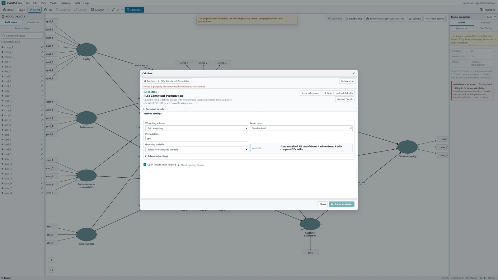
PLSc Consistent Permutation settings in QuickPLS. Select your own dataset and model, then use the choices described in the steps. Enter the practice permutation plan
Set Permutations to 1000. The standalone procedure accepts 99 to 10000 assignments. In Advanced settings, set Seed to 20261105 and record Parallel workers. The visible comparison is a fixed two-sided 5% test; there is no direction selector to change for this exercise. If interpreting a directional tail in a research study, justify that question before looking at the group results. Workers change computing capacity, not the hypothesis.
What you should see: The permutation count and seed are recorded.
How to read it: Keep the hypothesis and tail rule with the result.
Inspect the corrected fits behind the comparison
Review Readiness and click Start calculation. Labels are shuffled without replacement: each pooled case is assigned once in a given permutation, and the original group sizes are preserved. Each assignment fits PLSc afresh for both groups, including the measurement-error correction. In Results, inspect PLSc consistent permutation accounting and PLSc consistent-permutation failed assignments for requested, attempted, usable and failed counts. The procedure is not simply comparing the original fixed scores.
What you should see: The corrected group and reference fits are usable.
How to read it: Failures require diagnosis before a group-difference conclusion.
Read the planned path difference
Find the Quality to Satisfaction estimate for A, the estimate for B and their difference. Other supported comparison families include corrected loadings, construct correlations, rho_A and R². A loading describes an item's relationship with its construct; rho_A assesses reliability; R² describes explained sample variation. This route does not supply a general set of indirect-effect comparisons, bootstrap confidence intervals or automatic adjustment for many simultaneous tests.
What you should see: The planned path difference has a direct comparison result.
How to read it: Read it with both original group estimates.

Worked interpretation: from two coefficients to a permutation probability
Suppose the coefficient is 0.50 in A and 0.20 in B. A minus B is 0.30, so the estimated relationship is greater in A. If 39 of 999 usable shuffled assignments have an absolute difference at least 0.30, the two-sided add-one probability is (39 + 1)/(999 + 1) = 0.04. The comparison includes ties that are equally extreme. Adding one to both the count and denominator prevents a finite set of random assignments from producing a reported probability of zero.
Reverse the group order and the descriptive difference becomes -0.30. For the same cases, model and set of shuffled label assignments, the two-sided probability is preserved while the greater-than and less-than tails exchange places. A directional conclusion therefore needs the real group labels. Saying only that A was greater conceals which setting was compared with which.
At least 90% of planned assignments must be usable, and failed fits are not replaced. If 1000 assignments were planned but only 850 succeeded, the inferential calculation is unavailable. When a result is available despite some failures, its denominator uses the usable assignments. Report both that conditional calculation and the failures; do not rename the usable count as the planned count.
Even a small probability does not establish that the groups understood the indicators in the same way. A coefficient difference caused by changed measurement is a different finding from a difference in the structural relationship. Examine comparability before giving the contrast a substantive explanation.
Resolve group setup and measurement problems first
If the calculation is blocked, begin with the grouping column and group counts. A column already used as an indicator cannot also define these groups. Counts must be checked after rows missing required model values have been excluded, not just from the original spreadsheet totals.
If corrected fits fail after shuffling, examine reliability corrections, indicators with little variation and whether the corrected relationships form a mathematically valid matrix. Adding replacement assignments would hide the difficulty rather than resolve it. Preserve the failure information and use the table to select the next investigation.
If the estimates are valid but their difference is uncertain, report that uncertainty. Looking through many paths until one has a small probability creates a different analysis from testing the prespecified Quality to Satisfaction comparison.
On a small screen, swipe the table sideways to see every column.
| Symptom | Check | Reasonable action |
|---|---|---|
| Grouping variable is rejected | Whether it is also used as an indicator | Remove it from measurement blocks and retain it only as the grouping field. |
| A selected group has too few cases | Complete-case counts after model-specific exclusions | Review the sampling and missing-data plan. Do not merge substantively different groups solely to pass the minimum. |
| Corrected fits fail in shuffled groups | Reliability correction, whether the corrected matrix is mathematically valid, and indicators with little variation | Investigate unstable measurement and report failures; extra replacement permutations are not a remedy. |
| Two separate path tests look different | The actual A minus B comparison | Interpret the difference test. Separate significance labels are not a test of group difference. |
| Many parameter differences are highlighted | How many hypotheses were inspected | Define which hypotheses you will assess together and use a suitable broader analysis when adjustment is needed; this standalone route does not adjust them automatically. |
Check the direction and the assumptions behind label shuffling
As a direction check, reverse A and B while retaining the same cases, model and resampling plan. The sign should reverse and the directional questions should exchange places. A larger permutation plan chosen in advance can improve the resolution of a borderline probability; it cannot make the observed difference larger or add information to a small group.
Label shuffling needs an exchangeability assumption. In everyday terms, under the null model being tested, the reassigned labels must create a meaningful reference comparison. Dependence between cases, incompatible group distributions or a measurement model with different meanings can undermine that interpretation. More assignments do not fix those issues or severe group imbalance.
Review the group definition and measurement-comparability evidence before deciding which parameters belong in the planned comparison. If the study needs more than two groups, several adjusted comparisons or a combined invariance workflow, choose the appropriate broader analysis. Repeating standalone tests does not automatically control their collective false-positive risk.
Report the groups, their difference and the reference calculation
Methods example: We compared the same reflective model in groups 0 and 1 using PLSc permutation, with standardized complete-case data and Path weighting. Group 0 was A and group 1 was B. The two-sided comparison used 1000 planned label permutations and seed 20261105, preserving group sizes and refitting the corrected model within each assignment. Replace the numeric group codes with meaningful names and add actual complete-case, attempted, usable and failed counts.
Hypothetical Results example: The Quality to Satisfaction coefficient was 0.50 in A and 0.20 in B, a difference of 0.30. The two-sided probability was 0.04, calculated from 999 usable assignments. For the 1000-assignment plan in this example, that leaves one failed assignment; report its actual reason rather than inventing one. Interpreting the structural difference also requires separate evidence that the measurements were comparable across groups.
If you interpret a planned directional question, name the selected tail and the actual groups. Use the table below to keep the comparison, its calculation and the measurement evidence together.
| Report item | Detail to retain |
|---|---|
| Groups | Actual labels, A/B order and complete-case counts |
| Measurement | Common specification and separate comparability evidence |
| Model | PLSc corrections, weighting and scaling |
| Permutation | Planned, attempted, usable and failed assignments; seed |
| Comparison | Parameter, signed difference, alternative and probability definition |
Can you explain the group difference?
- Explain why a significant path in A and a nonsignificant path in B do not by themselves establish a difference between the paths.
- Calculate A minus B and state which real group has the greater estimate, keeping both original coefficients in view.
- Reconstruct the add-one probability from the extreme count and usable count, including equally extreme ties.
- Identify the separate evidence needed to show that the measurement is comparable between the groups.
- Explain when this standalone two-group procedure answers the question and when a broader multigroup or adjusted analysis is needed.