 QuickPLS
What the method does
Consistent bootstrapping applies the PLSc estimation procedure to resampled cases. Re-estimating the correction is essential because uncertainty also arises from the reliability and correlation estimates used by PLSc. Invalid corrected solutions must be accounted for when interpreting the resulting intervals.
For each resample b: fit PLS → estimate reliabilities → correct correlations → obtain θ*ᵦ.
The distribution of the usable corrected estimates θ*ᵦ supplies uncertainty for the PLSc quantity. It should not be replaced by an ordinary PLS interval attached to a corrected point estimate.
Data and analysis in QuickPLS
Use an eligible reflective PLSc model and the original cases. Check correction reliability and admissibility in the original fit before requesting resampling.
QuickPLS provides matching consistent-bootstrap results, including the requested and usable draw information. Inspect failed corrections before relying on the intervals.
Follow a worked example
The following example shows the data, settings and decisions for one analysis. Use the linked practice files to follow it. For your own study, keep the procedure and choose the variables, model and settings that fit your research question.
Download research-workshop.csv to begin. It contains 360 rows and 31 columns. The example below identifies the variables to use, their roles and any rows to exclude; not every column is an analysis variable.
Use the bootstrap that matches your PLSc estimate
Consistent PLS, usually shortened to PLSc, adjusts PLS estimates for measurement error under a common-factor model. A common factor is an underlying concept, such as satisfaction, treated as the reason its questionnaire items vary together. If you use this correction for the original estimate, you need to repeat it when assessing that estimate's uncertainty.
PLSc bootstrapping draws participant rows with replacement and fits the corrected model again for each sample. It repeats the measurement and structural calculations, not just the final path equation. Attaching an ordinary PLS interval to a PLSc coefficient would combine two different calculations.
Some resamples can produce a correction that is not mathematically valid even when the original model fitted successfully. Check these failures alongside the interval. Percentile, bias-corrected and accelerated (BCa), and studentized intervals each have additional requirements, so availability can differ between methods and statistics.
Practice: bootstrap a common-factor model
Suppose you treat Quality, Trust, Satisfaction and Loyalty as underlying concepts reflected in survey answers. PLSc is relevant when that common-factor interpretation and its assumptions fit the study. Its bootstrap repeats the correction in each sample, allowing the uncertainty introduced by the correction to enter the result.
Download the research workshop file and create the four reflective constructs with three matching indicators each. Draw Quality → Satisfaction, Trust → Satisfaction and Satisfaction → Loyalty. Start with complete data, Standardized results and Path weighting. Leave identifiers, group labels and weight outside the model.
The rows are independent synthetic cases for learning the workflow. These invented indicators are not a validated scale. The interpretation numbers below are hypothetical and are not fitted values from this download; inspect and report the output of your own exercise separately.
Begin with an interpretable corrected solution
Use a reflective model: each indicator is treated as an expression of its construct. Check the item coding, reliability corrections and the corrected relationships between constructs in the original PLSc result. A mathematically inadmissible correction is one that cannot represent a valid solution under this method; investigate it before asking for confidence intervals.
Keep the original model and data preparation available. In the exercise below, use standardized data, complete cases and Path weighting. Standardization expresses variables on a comparable scale; complete-case handling keeps only rows with all required model values. The weighting scheme is the rule used to form the construct scores before correction.
Write down the paths or indirect effects you want to assess, the confidence level and the test direction before viewing the bootstrap. This makes it easier to separate your planned analysis from useful follow-up exploration.
Choose the PLSc bootstrap settings
Use the workshop model’s own PLSc setup. Check Path weighting and Standardized result data, enter the teaching sample count below and expand Advanced settings to record its seed. Keep the point and bootstrap results separately identifiable.
Open the corrected bootstrap calculation
Choose Calculate, then PLSc Consistent Bootstrapping. Check that the selected model is the reflective PLSc model you intend to analyse. Every usable resample will repeat its consistency correction.
Set the sample count, confidence and hypothesis
Enter Bootstrap samples and Confidence level (%). Under Hypothesis test, choose Two-sided unless you planned a directional question. The directional choices are One-sided: greater than zero and One-sided: less than zero. Under Confidence intervals, choose Percentile and BCa for the practice run.
Add nested intervals only when they are needed
Also compute studentized intervals adds another bootstrap inside each outer sample. It reveals Inner samples per bootstrap sample, which takes an odd number from 99 to 999. Open Advanced settings to record Seed and Parallel workers. A one-sided hypothesis test still accompanies two-sided confidence intervals at the chosen confidence level.
Calculate and inspect availability
Choose Start calculation. In Results, read the corrected original estimate, its available intervals, and attempted, usable and failed counts. Read any reason given for an unavailable interval. Keep that explanation in your report instead of silently substituting a different method.
Run the full corrected bootstrap step by step
Check the original PLSc result
Fit the PLSc model first. Each reflective construct needs at least two indicators for this calculation; the exercise uses three. Check convergence, reliability corrections and the corrected construct correlation matrix, which is the table of relationships between constructs after correction. If that table cannot represent a valid set of relationships, investigate the model before resampling.
What you should see: The original corrected model is admissible.
How to read it: Check its reliability and corrected correlations first.
Enter the outer resampling plan
Choose PLSc Consistent Bootstrapping. Set Bootstrap samples to 1000 and Confidence level (%) to 95. The control accepts 1000 to 10000 samples. Keep the same complete-case model, Standardized result data and Path weighting. Factor weighting is also supported, but use it only as a deliberate, recorded change; PCA weighting is unavailable for this method.
What you should see: The outer resampling plan specifies the intended draws.
How to read it: Consistent correction must be repeated within each sample.
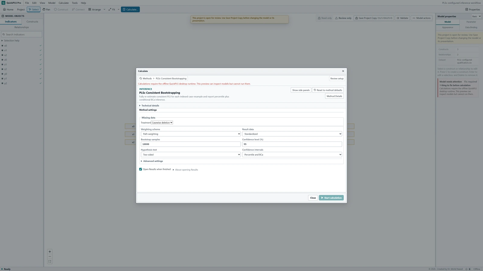
PLSc Consistent Bootstrapping settings in QuickPLS. Select your own dataset and model, then use the choices described in the steps. Choose the planned hypothesis
Under Hypothesis test, choose Two-sided for the exercise. This tests departures from zero in either direction. One-sided: greater than zero and One-sided: less than zero are for directions justified before seeing results. The confidence intervals remain two-sided whichever test you select. Read the probability's label rather than assuming it has the same definition as every interval beside it.
What you should see: The hypothesis and tail direction are explicit.
How to read it: Match the reported test to the research question.
Choose intervals and record the seed
Begin with Percentile and BCa under Confidence intervals. If a justified analysis calls for Also compute studentized intervals, set an odd Inner samples per bootstrap sample count from 99 to 999. In Advanced settings, set Seed to 20261105 and record Parallel workers. Workers control how many calculations can run together; they are a computing choice, not a research hypothesis.
What you should see: The interval choice, confidence level and seed are recorded.
How to read it: Nested procedures also need their inner-draw settings.
Check the complete corrected refits
Review Readiness and click Start calculation. In Results, select the completed PLSc bootstrap and inspect attempted, usable and failed samples. Each outer sample refits the PLS weights, reliability corrections and corrected structural relationships. Read the availability message for each path or effect you intend to report. Export those rows, their interval names and the PLSc settings together so that uncertainty remains attached to the corrected estimate that produced it.
What you should see: The completed output reports usable corrected refits and failures.
How to read it: Interpret intervals only where the requested inference is available.
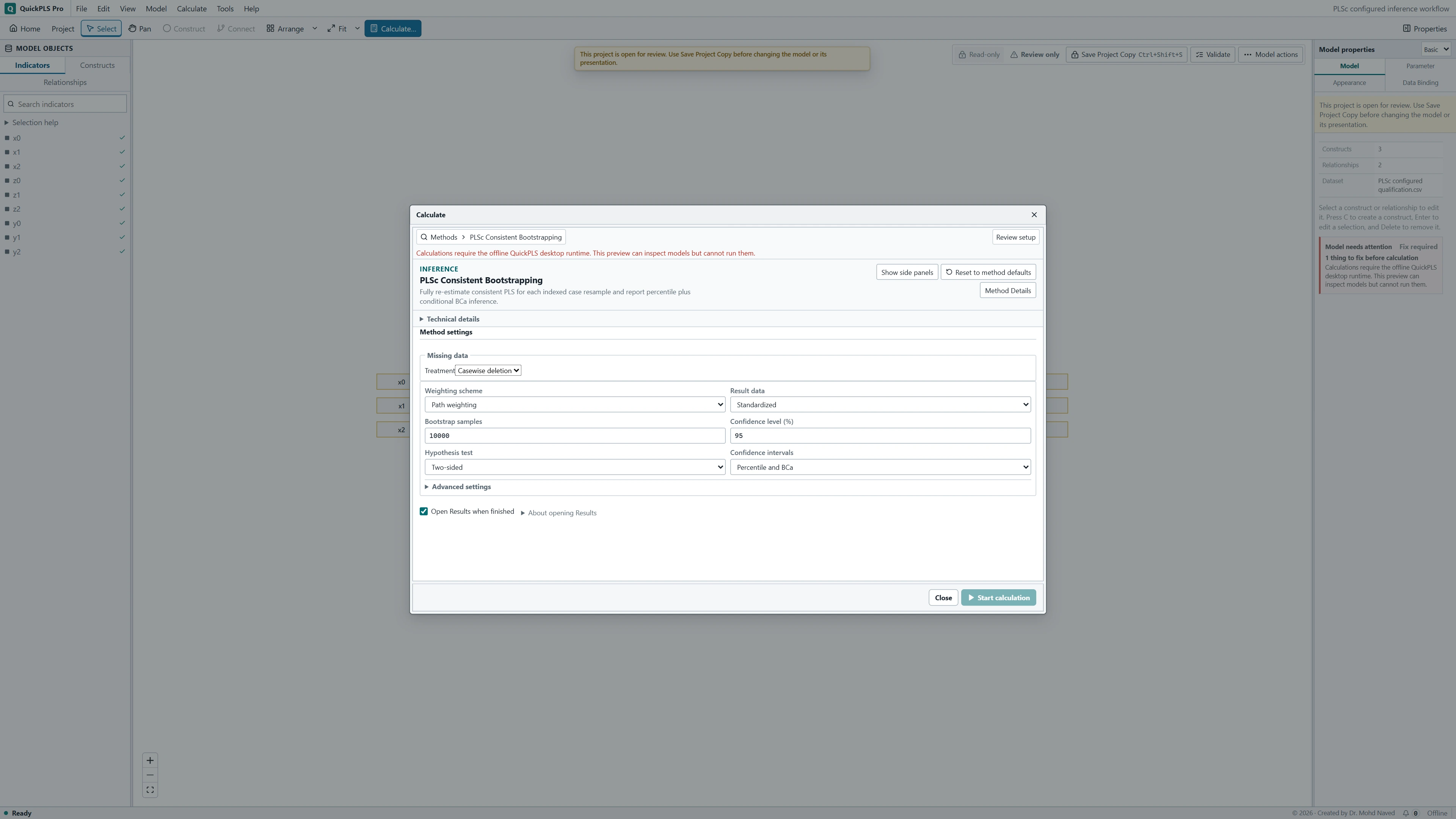
Read corrected estimates with their own uncertainty
Begin with the original corrected coefficient. The bootstrap mean averages the corrected estimates from usable resamples; the standard error describes their spread. A difference between the mean and original estimate is reported as bootstrap bias. It is a diagnostic feature of this calculation, not a reason to replace the original coefficient with the mean.
A percentile interval takes cut-offs from the corrected resampled estimates. BCa adjusts those cut-offs using both the bootstrap and a jackknife, which refits the model while leaving out each case in turn. Studentized intervals use a statistic scaled by its estimated uncertainty. That scaled statistic is called a pivot; the nested fits must provide a usable standard error before it can be formed.
Read the selected hypothesis-test probability separately from the interval. Two-sided asks whether a path differs from zero in either direction. A directional test asks about a positive or a negative path specified in advance. The interval remains two-sided, so a directional probability and an interval endpoint can appear to give different borderline decisions without being the same calculation.
In Results, use Search result outputs to find PLSc consistent bootstrapping, Bias-corrected and accelerated intervals and PLSc bootstrap replicate accounting. If requested, inspect Studentized confidence intervals and PLSc nested-refit evidence. Read the usable and failed outer samples, required jackknife fits and statistic-specific unavailable reasons. Keep those reasons with the effect rows.
On a small screen, swipe the table sideways to see every column.
| Output | How to read it | What to check |
|---|---|---|
| Corrected original estimate | The original corrected coefficient or other PLSc result whose uncertainty is being assessed. | Do not pair it with a PLS-only bootstrap interval. |
| Percentile, BCa and requested studentized intervals | Intervals from repeated corrected fits, with further resampling inside each outer sample for studentization. | Check the interval method, confidence level, usable standardized bootstrap statistics (pivots) and any missing interval. |
| Correction failures | Resamples in which the correction did not meet its mathematical requirements. | Report failed corrections rather than replacing or hiding them. |
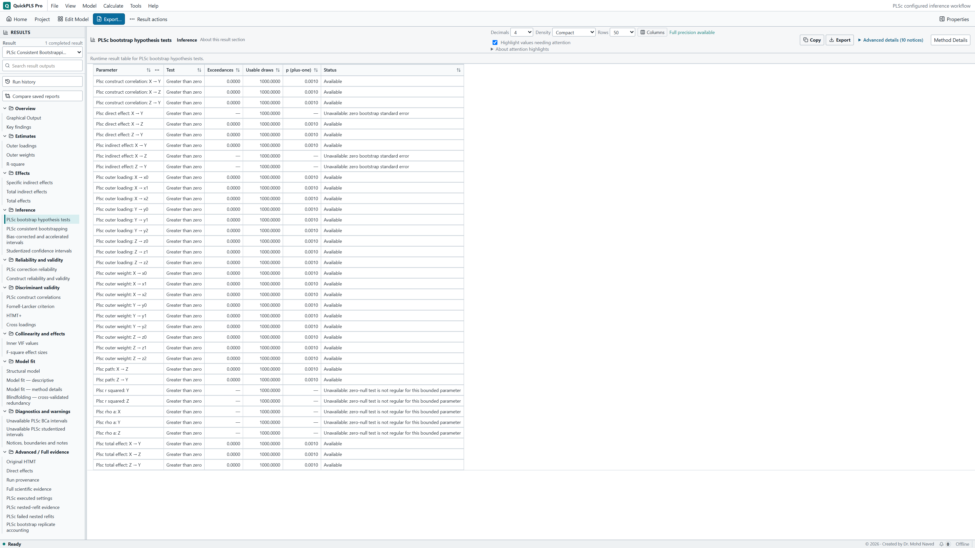
A narrow interval needs usable corrected fits behind it
An interval summarises the fits that met the calculation's requirements. Before calling it precise, check how many planned fits contributed and why others failed. Mathematical admissibility means that a corrected fit satisfies the method's requirements; it is separate from whether the research hypothesis was supported.
The usable-sample rule is a minimum requirement for calculation. Passing it does not remove the need to explain failures or evaluate the measurement model.
Illustrative example, not a software benchmark
A narrow interval based on a small usable subset of many attempted corrections needs investigation. Requesting more draws may reduce simulation noise, but it cannot resolve the measurement or admissibility problem causing the failures. Report the usable subset and the reason for concern.
Describe the corrected model and its bootstrap together
- Explain why the constructs are treated as common factors, identify their indicators and describe the original PLSc solution and correction checks.
- State the outer sample count, seed, confidence level, exact interval methods and selected hypothesis direction. If you requested studentized intervals, also give the inner sample count.
- Report attempted, usable and failed corrected fits, with failure reasons and unavailable statistics. Export these details with the original corrected estimates.
What more bootstrap samples can and cannot improve
More draws can make a finite simulation more stable. They cannot turn an invalid correction into a valid one or supply measurement information absent from the participants' responses. If the original correction fails, return to coding, item meaning and model specification first.
Keep PLSc estimates with PLSc uncertainty. Choosing ordinary PLS because its result appears to support a preferred hypothesis changes the estimator and its measurement assumptions. A justified comparison between estimators can be useful, but each result needs its own explanation and resampling procedure.
Worked interpretation: the correction and the usable-sample rule
Suppose the corrected Quality → Satisfaction coefficient is 0.38 with a hypothetical 95% percentile interval of [0.16, 0.60]. The range supports a positive corrected association under the PLSc assumptions, with substantial uncertainty about its size. A separate ordinary PLS calculation might give 0.31. That difference is not automatically an error: the estimators use different measurement assumptions and PLSc applies a correction. Keep each estimate with its own interval.
Suppose 1000 samples were attempted, 920 supplied usable corrected fits and 80 failed. The procedure requires at least 90% usable samples, so this example meets the numerical requirement. With 880 usable samples it would not. Passing the requirement does not make the 80 failures unimportant. Describe whether reliability corrections, unstable equations or other identified problems caused them.
BCa adds leave-one-case-out corrected fits. If a required jackknife fit fails, BCa can be unavailable even though percentile intervals exist. Studentized intervals add nested samples: 1000 outer samples with 99 inner samples require 99,000 inner fits. An outer estimate can remain usable even when its inner fits cannot supply a stable standard error for a particular statistic.
A path test against zero asks whether a relationship is supported under its null hypothesis. The same test is not automatically meaningful for every assessment measure. The reliability measure rho_A estimates the consistency of a construct's indicators; R² describes the share of an outcome's variation explained in the fitted sample. A missing path-style zero-null test for rho_A or R² does not mean that either value is zero. Read those measures using their own assessment and inference definitions.
Use the failure message to decide what to investigate
If the original PLSc correction is invalid, check coding and measurement before requesting another bootstrap. Weak items may supply little information about a factor; nearly duplicate items or predictors can make parts of the model unstable. A larger resample count cannot correct either problem by itself.
When only an interval is unavailable, identify which extra calculation it needed. BCa depends on the corrected jackknife; studentization needs usable inner fits and a nonzero standard error. Keep the available result under its correct name. The table below separates these situations from a test whose result simply does not support the planned direction.
On a small screen, swipe the table sideways to see every column.
| Symptom | Check | Reasonable action |
|---|---|---|
| The original PLSc correction is invalid | Reliability correction and corrected correlation matrix | Review measurement specification and coding before attempting inference. Do not bootstrap an invalid point solution. |
| More than 10% of planned samples fail | Failure categories and weak or redundant indicators | Investigate the unstable correction and report the unavailable result. The procedure does not replace failed draws to meet the required count. |
| Percentile is present but BCa is absent | Corrected jackknife fits | Use precise interval naming and disclose the unavailable method rather than relabelling the percentile interval. |
| Studentized interval fails | Inner fit counts and nonzero standard errors | Review the inner resampling results. A larger inner plan may improve simulation precision but cannot make an invalid model valid. |
| One-sided probability seems inconsistent with the interval | Selected hypothesis direction and two-sided interval definition | Report both definitions. Do not quietly reinterpret a two-sided interval as a one-sided bound. |
Evaluate the assumptions before comparing probabilities
Start from what the construct represents. In a common-factor model, the underlying concept is used to explain why its items move together. A composite is deliberately formed from its components. These are different measurement ideas; choose an estimator to match that idea before comparing p-values from different estimators.
For a numerical sensitivity check, keep the data and model fixed and use a declared larger outer plan or a justified alternative interval procedure. Record failures for every comparison. A result that repeatedly changes its conclusion around zero is uncertain, even if one setting happens to give the preferred decision.
Correct documented data errors and rerun the original and bootstrap calculations. If you revise the indicators or paths for a substantive reason, preserve the previous result and explain the change. Increasing draws alone cannot create stronger measurement or additional participants.
A methods paragraph and a results paragraph to adapt
Methods example: We estimated the reflective model using consistent PLS with standardized data, complete-case handling and Path weighting. We attempted 1000 case-bootstrap samples with seed 20261105, repeating the measurement and structural corrections within each sample. We requested 95% percentile and BCa intervals and selected a two-sided hypothesis test. Replace these settings with those actually used, and add the sample size and common-factor rationale.
Hypothetical Results example: The corrected Quality to Satisfaction coefficient was 0.38, with a 95% percentile interval of [0.16, 0.60]. Of 1000 attempted samples, 920 provided usable corrected fits and 80 failed. We reported their causes and the availability of the requested intervals. These numbers illustrate reporting; they do not claim that the downloadable practice data produced this result.
If you requested nested analysis, add the inner sample count and report unavailable statistics with their reasons. State the selected hypothesis direction even though the intervals are two-sided. Use the table to check that the reader can identify both the corrected model and the uncertainty procedure.
| Report item | Required detail |
|---|---|
| Measurement | Common-factor rationale and indicators per block |
| Estimator | PLSc, weighting, scaling and missing-data handling |
| Resampling | Outer count, seed, usable and failed fits |
| Inference | Hypothesis direction, confidence level and exact interval method |
| Nested analysis | Whether requested, inner count and unavailable statistics |
Can you explain a PLSc bootstrap without mixing estimators?
- Explain why an ordinary PLS bootstrap interval does not describe uncertainty for a corrected PLSc coefficient.
- Identify the score weights, reliability correction and structural relationships that are refitted in each corrected sample.
- Calculate the usable proportion from the actual counts and explain why meeting the requirement does not erase the failures.
- Explain why selecting a one-sided hypothesis test does not turn the reported two-sided interval into a one-sided bound.
- Report an unavailable BCa or studentized interval by name, with its reason, while keeping any available interval under its correct name.