 QuickPLS
What the method does
Interventional mediation defines effects by comparing outcome expectations under explicit treatment levels and mediator distributions. The target is an intervention-based contrast, not automatically the product of two regression coefficients. Interpretation depends on the intervention definition, adequate covariate adjustment and causal identification assumptions.
Illustrative indirect contrast: E[Y(a, Gₐ)] − E[Y(a, Gₐ*)].
a and a* are treatment levels. Gₐ denotes a draw from the mediator distribution under level a, as defined by the analysis. Holding treatment at a while changing that distribution isolates the specified interventional contrast. Conditional definitions and multiple mediators require the matching model assumptions.
Data and analysis in QuickPLS
Provide treatment, mediator, outcome and relevant covariate information for the supported model. Define the treatment contrast and intervention population before calculation.
QuickPLS provides the intervention settings, effect estimates and uncertainty. Check the stated contrast in each output row before interpreting or reporting it.
Follow a worked example
The following example shows the data, settings and decisions for one analysis. Use the linked practice files to follow it. For your own study, keep the procedure and choose the variables, model and settings that fit your research question.
Download observed-workshop.csv to begin. It contains 120 rows and 8 columns. The example below identifies the variables to use, their roles and any rows to exclude; not every column is an analysis variable.
What would change under the specified intervention?
Suppose a study asks what would happen to a later outcome if an exposure changed, and how much of that change would operate through intermediate responses. That is a causal question. Interventional Mediation estimates the defined comparison using equations fitted to directly observed variables. Its method, parametric g-computation, uses those equations to calculate expected outcomes under the specified conditions and then averages them.
The workflow supports one to three ordered continuous mediators and a continuous outcome. The treatment contrast states the two exposure values being compared. The adjustment variables are measured baseline variables used to account for common causes. Their choice, the mediator order and the treatment contrast all help define the question.
Positivity means that the treatment conditions being compared are supported across the relevant baseline circumstances. For example, there should be information about both conditions for the kinds of participants to whom the conclusion applies. Software can flag missing support, but it cannot establish that every important common cause was measured. Bootstrap resampling assesses sampling uncertainty after these modelling choices are made.
Write the intervention and causal argument in ordinary words
State what changing treatment means, which population you want to describe, the 1 to 3 ordered continuous mediators and the continuous outcome. Identify baseline adjustment variables and explain their roles before calculating. A baseline variable is measured before treatment and is not a consequence of it.
Confounding occurs when a common cause helps explain two variables' relationship. The identification assumptions concern relevant common causes of treatment and outcome, treatment and mediator, and mediator and outcome. Identification means that the stated effect can be learned from the observed data under those assumptions. Consistency additionally requires a well-defined intervention whose meaning matches the treatment being studied.
This workflow excludes a treatment-induced mediator-outcome confounder: a variable changed by treatment that then affects both the mediator and outcome. It also excludes a recanting-witness setting, where isolating selected causal paths would require an intermediate variable to carry incompatible treatment histories along different paths. These are design questions to review, not boxes the numerical result can settle.
Check whether the data contain observations relevant to both treatment values. The local support screen is a useful diagnostic, but the substantive comparison and the causal argument still need to make sense.
Set up the observed-data intervention analysis
Use observed-workshop.csv for the first exercise. Its columns are assigned directly in this setup; do not substitute scores from the PLS service model. Write the treatment change and causal assumptions before selecting roles, because the software can check the specification but cannot establish those assumptions for you.
Open the separate interventional workflow
Choose Calculate, select Interventional Mediation and continue to setup for the intended observed dataset. This is separate from a PLS indirect-path calculation and from the observed-variable PROCESS association model.
Define roles, paths and equations
Select Treatment, Continuous outcome, Treatment contrast, Observed continuous mediators and the Required nonempty adjustment set. Enter the Explicit causal paths with the variable identifiers shown by the app. Review the Explicit observed-data equations and Identification and positivity declarations, then set Bootstrap replicates.
Calculate and assess the requested comparison
Run the analysis once the setup is complete. Check treatment values, mediator order and observed support before reading direct, joint indirect and total effects. Read their matching uncertainty and bootstrap diagnostics. The interpretation remains conditional on the stated causal and equation assumptions.
Read the comparison and support checks before the effects
First confirm the treatment values and mediator order. A different treatment change or a different sequence of mediators describes a different intervention question. Read the direct, joint indirect and total contrasts using those definitions, not as generic labels borrowed from an ordinary PLS result.
Joint indirect means the effect associated with the declared change in the mediator distribution along the selected pathway. The output also reports observed-support checks and bootstrap diagnostics. A fitted equation can return a number even when a treatment condition is poorly represented in relevant participants. A narrow interval does not create the missing information or account for an unmeasured common cause.
The results are assumption-dependent interventional estimates. Check the effect definition, uncertainty and support together before deciding what the study can claim.
On a small screen, swipe the table sideways to see every column.
| Output | How to read it | What to check |
|---|---|---|
| Treatment contrast and ordering | The intervention comparison and mediator sequence being estimated. | Different contrasts or orders define different questions. |
| Joint interventional effects | Effects under the declared parametric g-computation specification. | State the assumptions required to interpret these estimates as causal effects. |
| Observed support / bootstrap diagnostics | Whether the data cover the requested treatment contrast and whether bootstrap calculations completed. | A numerically returned estimate does not overcome poor overlap. |
A precise fitted answer can still rely on extrapolation
Extrapolation means using the fitted relationship to predict a condition that has little or no relevant data behind it. For instance, a treatment level may be common overall but almost absent among participants with a particular baseline profile.
If that profile matters to the target population, reconsider the supported comparison and report the gap. A confidence interval addresses uncertainty under the fitted procedure; it does not prove that a missing treatment condition has been adequately represented.
Illustrative example, not a software benchmark
One treatment condition is almost absent for a relevant covariate pattern. The fitted model may have to extrapolate that intervention response. A narrow bootstrap interval does not remove the lack of support. Reconsider the contrast or target population before drawing a causal conclusion.
Practice: change x from 0 to 1 through one mediator
For this teaching scenario, let x be a controllable exposure, m an intermediate response and y a later continuous outcome. Ask how the expected outcome would differ when x changes from x0 to x1, including the change through the mediator distribution. That question needs a causal argument about timing, common causes and observed support; it is not obtained by renaming an ordinary indirect path.
Download observed-workshop.csv, which contains 120 synthetic cases. Assign x as treatment, m as the single continuous mediator, y as the continuous outcome and z as a baseline adjustment variable. Use the continuous contrast x0 = 0 to x1 = 1. Keep case_id, group, weight and binary_outcome outside this analysis.
These assignments define a practice scenario, not facts established by the file. In a real study, explain what a one-unit treatment change means and why z is a justified pretreatment adjustment. The synthetic data do not verify that z captures all confounding or that the intervention is well defined.
Specify the treatment, ordered path and equations
Write the causal sequence first
For the exercise, assume z was measured before x, x preceded m and m preceded y. Explain what changing x from 0 to 1 would mean. List plausible common causes of treatment, mediator and outcome. If a real study cannot defend the required assumptions, answer an associational question rather than treating the calculation as evidence that causality has been established.
What you should see: The treatment-to-mediator-to-outcome sequence is explicit.
How to read it: A diagram alone does not establish its causal assumptions.
Assign the observed-variable roles
Open Interventional Mediation and continue to setup. Choose x under Treatment and y under Continuous outcome. Select Continuous x0 → x1 under Treatment contrast and enter 0 and 1. Choose m under Observed continuous mediators and z under Required nonempty adjustment set. Leave baseline moderators unselected for this first exercise.
What you should see: Observed variables and adjustment roles are assigned correctly.
How to read it: Check outcome coding and treatment contrast.
Enter the ordered causal path
In Explicit causal paths, enter a named path using the actual identifiers displayed beside x, m and y. Follow the form path:exposure-mediator-outcome = treatment_id > mediator_id > outcome_id. Replace those example identifiers with the app's identifiers for x, m and y. The greater-than signs mark path order; they are not comparisons between numeric values. A column label need not be its internal identifier.
What you should see: The ordered causal path matches the intended intervention question.
How to read it: Keep the contrast direction with the result.
Check each staged equation
Under Explicit observed-data equations, specify m from x and z, then y from x, m and z. Read each Staged equation to confirm the terms. The intercept is included automatically; required predecessor and adjustment terms cannot be removed. Every adjustment variable belongs as a main effect in every equation. An outcome measured later cannot predict an earlier mediator in this ordered calculation.
What you should see: Each staged equation uses its intended predictors and cases.
How to read it: Investigate inadequate support before deriving effects.
Review assumptions and support honestly
Review Identification and positivity declarations: time order, a well-defined intervention, justified adjustment, the relevant unmeasured-confounding assumptions, excluded treatment-induced confounding and path settings, linear equations and positivity. A treatment-induced mediator-outcome confounder is caused by treatment and then affects both mediator and outcome. The declarations record your review; they do not prove the assumptions. Inspect the support findings for the actual treatment contrast.
What you should see: The assumptions and support review are recorded.
How to read it: A numerical estimate cannot compensate for an unjustified causal specification.
Request and inspect bootstrap uncertainty
Set Bootstrap replicates to 500 for practice; the control permits 500 to 10000. Choose Start calculation. In the completed result, inspect Identification assumptions and Positivity diagnostics before Interventional mediation effects. Read the returned inference settings, completion status, usable counts and failure reasons. Incomplete bootstrap inference leaves the corresponding intervals and probabilities unavailable. Save the effect definitions, equations, support diagnostics and declarations together.
What you should see: The completed result gives the named intervention effects and usable uncertainty.
How to read it: Report the contrast, assumptions and confidence bounds together.
Understand the three expected outcomes behind the effects
The observed linear method evaluates fitted average responses in mediator order, then averages over the observed baseline covariate values. A covariate is an adjustment variable. If a baseline moderator has an explicitly fixed value, that value is handled as declared. The point calculation uses fitted conditional means; it does not need a separate random simulation of mediator values. The bootstrap then estimates sampling uncertainty around this fitted analysis.
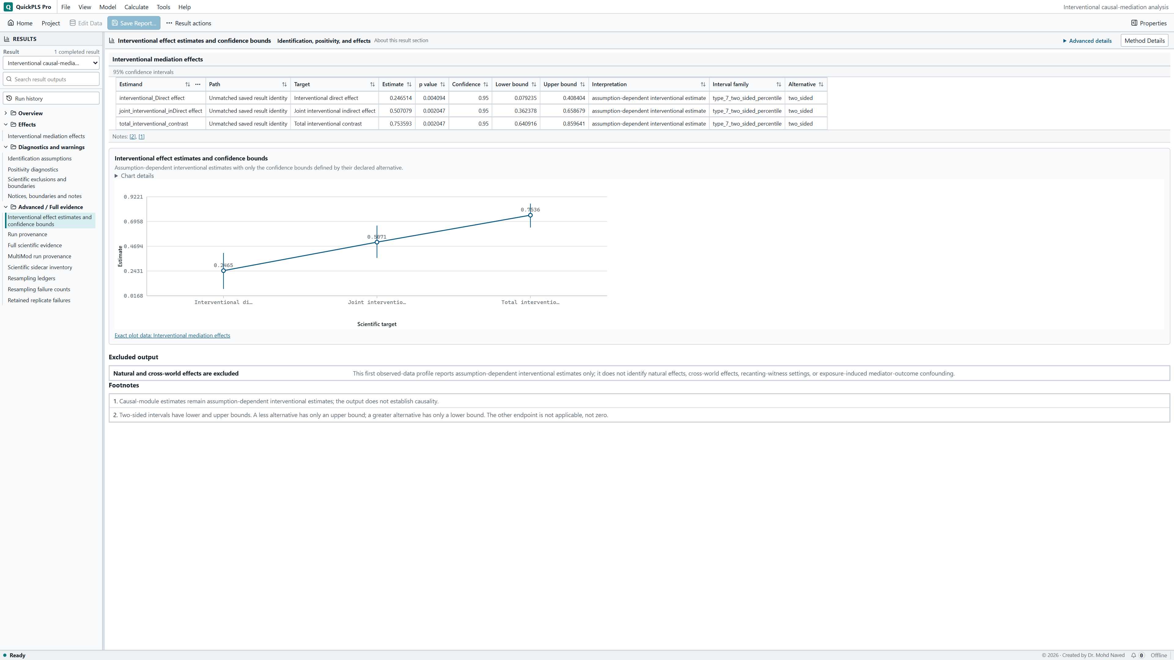
Three expected outcomes define the decomposition. mu00 uses treatment x0 and the mediator distribution under x0. mu10 changes treatment to x1 while keeping the mediator-distribution intervention under x0. mu11 uses treatment x1 and the mediator distribution under x1. Subtract mu00 from mu10 for the direct contrast, mu10 from mu11 for the joint indirect contrast, and mu00 from mu11 for the total. These names label the conditions being averaged, not three different datasets you must upload.
The joint indirect contrast concerns a defined change in the mediator distribution. It is not a natural indirect effect, which relies on the mediator value each particular person would have had under another treatment condition. With several ordered mediators, the joint result is not automatically the isolated contribution of each mediator. A separate contribution needs its own supported definition.
Work through the decomposition and support checks
Suppose the expected outcomes are mu00 = 2.00, mu10 = 2.30 and mu11 = 2.80. The direct contrast is 0.30, the joint indirect contrast is 0.50 and the total is 0.80. Direct plus joint indirect equals total. These are hypothetical arithmetic values, not estimates from the downloadable data.
If the hypothetical joint indirect interval is [-0.10, 0.90], its positive point estimate remains uncertain: the range includes zero and values in both directions. This does not show that the mediator is irrelevant. An interval excluding zero would still leave the study's confounding and intervention assumptions to be justified.
For a continuous treatment, x0 and x1 must be finite, different and within the observed range, with enough nearby observations. The default local screen requires five observations within five percent of that range around each value. Passing means there is observed local support. It does not establish overlap for every combination of adjustment variables or exchangeability, the assumption that relevant unmeasured common causes do not remain after adjustment.
For a binary treatment, all observed values must belong to the declared two arms, with the required counts and balance. An arm is one treatment condition. Optional declared baseline strata can require both arms within each stratum; a stratum is a subgroup defined by baseline characteristics. A nearly absent condition in an important covariate pattern cannot be repaired by extrapolating the fitted regression more confidently.
A separate check of the supplied CSV found x values from -2.314387 to 1.712648. Five percent of that span is approximately 0.201352. There are 17 observations within that distance of 0 and 18 within that distance of 1. This checks nearby observations for the teaching contrast only. It does not verify conditional overlap, the causal assumptions or a successful app analysis.
Separate a design problem from a fitting problem
If a causal assumption cannot be supported, reconsider the study question before changing numerical settings. If the contrast lacks support, consider a scientifically meaningful supported contrast or a transparently revised target population. Lowering a threshold merely to make the calculation run does not supply the missing information.
For fitting failures, inspect the equations. Duplicate terms or nearly dependent predictors can prevent unique estimates. Product terms need their component main effects and must follow the supported ordering. Use the table to decide whether to correct data, revise a model for a stated reason or choose a different method.
If only uncertainty is unavailable, inspect bootstrap completion and failed fits. A point estimate is not a substitute for an interval. If an available interval includes zero, report the uncertainty instead of removing adjustment variables to make it narrower.
On a small screen, swipe the table sideways to see every column.
| Symptom | Check | Reasonable action |
|---|---|---|
| An assumption cannot honestly be confirmed | Temporal order, intervention meaning and omitted common causes | Stop the causal interpretation and reconsider the design or report an associational question. |
| Contrast fails the support screen | Treatment range and nearby or arm-specific counts | Choose a scientifically meaningful supported contrast or redefine the target population transparently; do not merely lower thresholds until it runs. |
| Adjustment set is rejected | A nonempty baseline set and distinct variable roles | Choose justified pretreatment covariates and keep them in every equation; avoid adjusting for an effect of treatment as though it were baseline. |
| An equation cannot be estimated uniquely | Duplicated terms, strongly dependent predictors and observations relative to parameters | Correct errors or simplify for a substantive reason. Do not switch to another estimator without reporting the change. |
| A product term is unavailable | Hierarchy and the restriction to at most one post-treatment mediator per term | Use the supported equation specification or a different appropriate method; products of multiple mediators change the required mathematics. |
| Intervals are missing | Bootstrap completion and fit failures | Report the unavailable inference and diagnose it. A successful point estimate alone does not provide uncertainty. |
Explain what changes when you revise the intervention
A useful sensitivity exercise compares plausible, supported treatment contrasts or justified adjustment specifications while keeping the original result. Moving from 0 → 1 to another contrast changes the intervention. Removing z changes the confounding assumption, even if the interval becomes narrower. Explain each revision using the study's substantive question.
This analysis uses directly observed numeric variables, one to three ordered continuous mediators and a continuous outcome. Latent constructs, groups, case or frequency weights, natural effects, treatment-induced mediator-outcome confounding and unsupported causal pathways require a different appropriate analysis. Additional measurements or a stronger design may be needed. More bootstrap draws can refine sampling calculations; they cannot establish the causal assumptions.
Keep the causal argument, support and effects together
Methods example: We specified an observed-data interventional mediation analysis for the continuous treatment contrast x = 0 to x = 1, with ordered path x → m → y and baseline adjustment z. Linear mediator and outcome equations included intercepts and the adjustment variable. We calculated direct, joint indirect and total interventional contrasts from fitted conditional means averaged over the observed baseline distribution, with 500 bootstrap replicates for uncertainty. Add the actual identification argument, sample information, support findings and inference settings.
Hypothetical Results example: The direct, joint indirect and total contrasts were 0.30, 0.50 and 0.80. The direct and joint indirect parts summed to the total. These are assumption-dependent interventional estimates; the calculation does not establish causality. A real report must add the matching confidence intervals, usable and failed bootstrap counts and the findings from the support checks.
Use the table to confirm that readers can see which intervention and population the effects concern. Keep the joint indirect label unless a different effect was explicitly defined and estimated.
| Report item | Detail to include |
|---|---|
| Intervention | Treatment, x0, x1 and target population |
| Path and roles | Ordered mediators, outcome, baseline covariates and moderators |
| Equations | Main effects, interactions, intercepts and linearity assumptions |
| Identification | Timing, confounding argument and excluded problematic pathways |
| Support | Treatment ranges or arms, local counts and any strata |
| Effects | mu00, mu10, mu11, direct, joint indirect, total and matching uncertainty |
Can you explain the intervention and its assumptions?
- Describe what the selected treatment change would mean in the real study and which population it concerns.
- Write the two practice equations, showing z in both and the mediator order.
- Reconstruct the direct, joint indirect and total contrasts from the three expected outcomes.
- Explain why fitting expected outcomes and bootstrapping their uncertainty are separate steps.
- Explain why nearby observations in the support screen do not prove absence of unmeasured confounding.
- Report the result as an assumption-dependent joint interventional effect, without relabelling it a natural indirect effect.
Report the assumptions with the estimate they support
- Define the treatment change, target population, mediators in order, outcome and baseline adjustment variables.
- Explain the causal assumptions and the evidence from the support checks, including any important baseline patterns with limited overlap.
- Give the fitted equations, interval and bootstrap settings, usable or failed fits, and direct, joint indirect and total contrasts. Describe them as conditional on the stated assumptions.
State the design and assumptions behind a causal conclusion
The calculation does not establish causality by itself. This observed-data g-computation workflow answers a defined intervention question under assumptions about timing, confounding, support and the equations. It does not turn a PLS indirect association into a causal effect by changing its label.
If an assumption cannot be defended, a carefully reported associational analysis may still answer a useful question. A stronger design or additional measurements may be needed before interpreting the pathway as an effect of an intervention.