 QuickPLS
What the method does
CB-SEM model comparison asks whether a less restrictive model improves fit enough to justify its extra parameters. A likelihood-ratio difference test applies to appropriately nested models fitted with compatible estimators. Information criteria provide a different comparison of fit and complexity; they do not turn non-nested models into a nested test.
Nested comparison: Δχ² = χ²restricted − χ²free; Δdf = dfrestricted − dffree.
The restricted model imposes constraints contained in the more general model. Under the relevant regularity conditions, the difference is assessed using its difference in degrees of freedom. Robust or scaled statistics require their corresponding difference procedure rather than simple subtraction.
Data and analysis in QuickPLS
Use two saved, identified CB-SEM models with the same analysed cases, variables and compatible estimation settings. State the restriction that makes them nested, if requesting that test.
QuickPLS compares the selected saved models and reports their fit and comparison results. Check model names, sample consistency and the tested restriction before choosing an interpretation.
Follow a worked example
The following example shows the data, settings and decisions for one analysis. Use the linked practice files to follow it. For your own study, keep the procedure and choose the variables, model and settings that fit your research question.
Download research-workshop.csv to begin. It contains 360 rows and 31 columns. The example below identifies the variables to use, their roles and any rows to exclude; not every column is an analysis variable.
Test the direct Quality-to-Loyalty path
Suppose your model says that Quality is related to Loyalty through Satisfaction. You also want to test a direct Quality-to-Loyalty path. Save a model that estimates that path and a second model that fixes its coefficient to zero. The comparison asks how much worse the model describes the data when that one relationship is removed.
This is a nested comparison: the simpler model is the larger model with a stated restriction. A likelihood-ratio test checks the loss of fit caused by that restriction. Degrees of freedom count the independent restrictions in the fitted model; different counts alone do not establish that two models are nested.
For comparable models that are not nested, use the Akaike information criterion (AIC) and Bayesian information criterion (BIC) instead. These criteria balance fit against the number of estimated parameters. Lower values favour a model within the pair, provided both values describe the same data and use compatible likelihood and parameter-count definitions. They do not establish that the chosen explanation is true.
Save two models that differ only where intended
Use the same dataset, analysed rows, observed variables and variable order in both models. Keep the measurement model, factor scaling, treatment of means and missing-data rule the same. For a nested test, write down the exact restriction before calculating. Both fits must use ordinary maximum likelihood, the estimation method used in this guide. It chooses model parameters that make the observed data most plausible under the model.
In the comparison screen, Model A — unrestricted must be the saved model that estimates Quality → Loyalty. Model B — restricted must fix that same coefficient to zero. Check the file and model descriptions before starting.
Choose the pair and run the comparison
Open the comparison screen
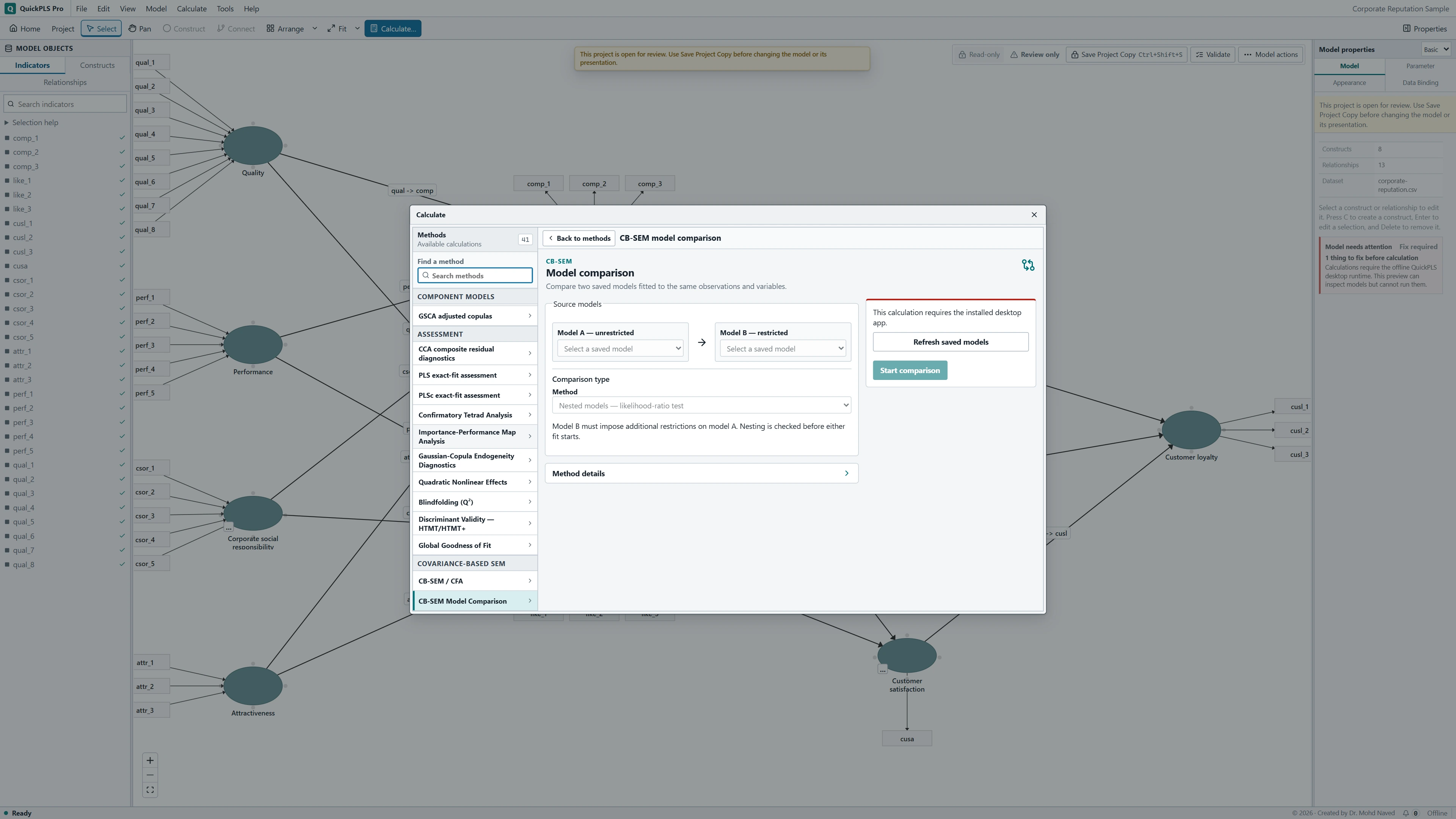
Click Calculate… and find CB-SEM Model Comparison in the method list. Under Source models, choose the model with the direct path in Model A — unrestricted. Choose the model that fixes that path to zero in Model B — restricted. If a newly saved model is missing, click Refresh saved models.
Choose the question you want to answer
Under Method, choose Nested models — likelihood-ratio test for this restriction. The app checks the nesting before fitting the pair. Use Descriptive comparison — AIC and BIC only for the separate question of comparing compatible models without a nested significance test.
Calculate, then open the saved result
Click Start comparison. When it finishes, click Open Results. Read Model fits and the restriction information before interpreting Nested model comparison. In descriptive mode, read Descriptive model comparison and its stated subtraction direction.
Check the models before reading the difference
After Open Results, use Search result outputs to find Model fits. Check the common sample, the fit of each model and its number of estimated parameters. Then open Nested model comparison. Chi-square summarises the mismatch between the model and observed data. The chi-square and degrees-of-freedom differences are restricted Model B minus unrestricted Model A.
For Descriptive model comparison, the AIC and BIC differences run the other way: Model A minus Model B. A negative difference favours A for that criterion. Read the heading and direction each time; a negative AIC difference is not a negative likelihood-ratio statistic. The table below explains the roles of these outputs.
On a small screen, swipe the table sideways to see every column.
| Output | How to read it | What to check |
|---|---|---|
| Restriction / nesting evidence | Which parameters are fixed or constrained in the restricted model. | Do not infer nesting solely from fit statistics. |
| Likelihood-ratio difference | How much fit worsens when the specified restrictions are imposed. | Check nesting, identical observations and variables, and compatible maximum-likelihood definitions. |
| AIC / BIC | Criteria that balance fit and model complexity using the stated likelihood calculation. | A smaller criterion does not prove causal correctness. |

Changing a path and changing a questionnaire answer different questions
Ask yourself what the simpler model says. Fixing the direct path to zero says that Quality has no additional direct association with Loyalty after accounting for the other paths. Replacing an indicator instead changes what is measured. Use the example below to check that your pair tests the question you intended.
Illustrative example, not a software benchmark
Removing a structural path can produce a nested model if the rest of the specification and the observations stay the same. Replacing indicators changes the variables being modelled. That second comparison cannot be treated as the same restriction test, even if the diagrams look similar.
Practice: keep or remove the direct Quality-to-Loyalty path?
Download research-workshop.csv below. It contains 360 synthetic cases for practising the workflow. Build Quality from quality_1 to quality_3, Trust from trust_1 to trust_3, Satisfaction from satisfaction_1 to satisfaction_3, and Loyalty from loyalty_1 to loyalty_3. For each construct, use Properties → Inspector mode Expert → Parameter, set Measurement model to Reflective and Scientific representation → Representation to Common factor. Choose its first indicator as Marker indicator: quality_1, trust_1, satisfaction_1 or loyalty_1. These invented scores are teaching data, not a validated service questionnaire.
Draw Quality → Satisfaction, Trust → Satisfaction and Satisfaction → Loyalty. Then add Quality → Loyalty to the unrestricted model. This last arrow represents the additional direct association you want to test. Add a covariance between the exogenous Quality and Trust factors: select their connection, set Relationship type to Covariance and Relationship use → Use to Model covariance, then choose Apply relationship use. Do not add cross-loadings or residual covariances for this exercise. Give the model a name that identifies it as unrestricted.
Create a separate saved specification in which the Quality → Loyalty coefficient is fixed to zero. Keep all four factors, every indicator and all other assumptions unchanged. Both models must use the same complete cases: rows with all the values required by this analysis.
Build, check and compare the two specifications
Check the model with the direct path
Fit the unrestricted model using CB-SEM / CFA. Choose Estimation workflow → Continuous-linear structural ML, Moment structure → Covariances and Inference → Maximum-likelihood point estimates. This covariance-only exercise does not estimate a mean/intercept structure. Confirm that the fit converged, meaning that its estimation updates settled within the stopping criterion. Check the first-indicator markers and look for impossible estimates such as negative residual variances. Record the analysed cases and indicator order.
What you should see: The less restricted model contains the direct path.
How to read it: Retain its fit and exact analysed cases.
Fix the direct coefficient in a separate model
In the restricted specification, open Model → Advanced Relationships and Parameters…. Find the Quality → Loyalty parameter and click Edit. Set Specification to Fixed, enter 0 in Fixed value and click Apply. Save the restricted model separately, keeping its factor scaling, covariance or mean structure, data and missing-data rule unchanged. Fit it and check that its estimates are usable too.
What you should see: The comparison model fixes that coefficient as stated.
How to read it: Its restriction must be contained within the less restricted model.
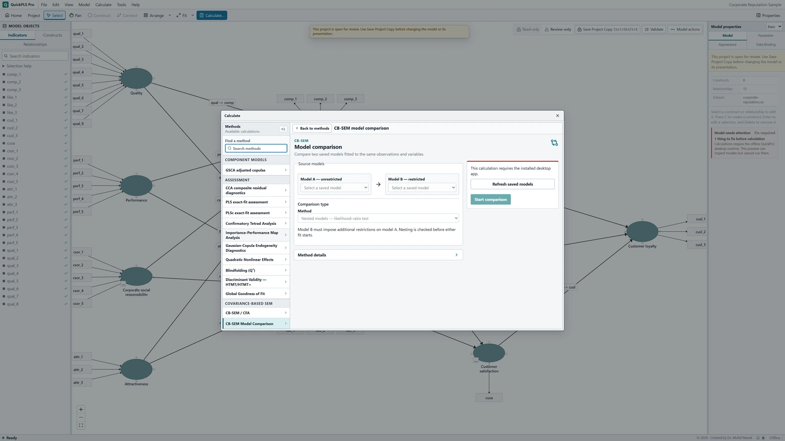
CB-SEM Model Comparison settings in QuickPLS. Select your own dataset and model, then use the choices described in the steps. Select A and B by name
Open Calculate… → CB-SEM Model Comparison. Under Source models, select the unrestricted specification as Model A — unrestricted and the zero-restriction specification as Model B — restricted. Match the dataset descriptions as well as the model names.
What you should see: The setup names A and B in the intended order.
How to read it: Reverse labels would change the direction of reported differences.
Select the nested test
Choose Nested models — likelihood-ratio test under Method. This is the test for the declared zero restriction. Descriptive comparison — AIC and BIC is a separate option for a comparable non-nested pair; it does not supply a non-nested significance test.
What you should see: The selected nested test corresponds to the declared restriction.
How to read it: Use another comparison if the models are not nested.
Run and inspect both fits
Click Start comparison, then Open Results. Search for Model fits and Nested model comparison. Check that the restricted model has the additional restriction and larger degrees of freedom before reading the difference statistic.
What you should see: Both fits and their difference are available for compatible cases.
How to read it: A failed fit cannot support a valid nested comparison.
Save the whole comparison
Keep the model specifications, both fit summaries and the comparison together. If the app rejects the pair, read and resolve the named mismatch. Changing the comparison option does not repair a mismatch in the data or create a valid nested test.
What you should see: The saved record includes both models and the test.
How to read it: Report the restriction and model order with the conclusion.
Work through the difference, then consider its size
These are hypothetical teaching values, not the answers for the downloaded CSV. Suppose unrestricted Model A has chi-square 120.0 on 50 degrees of freedom and restricted Model B has 125.0 on 51. Subtract A from B: the loss of fit is 5.0 on 1 degree of freedom. Its ordinary chi-square upper-tail probability is approximately 0.025. Under the model assumptions, this is evidence against fixing the direct coefficient to zero.
Next read the direct coefficient and its uncertainty. Detectable loss of fit does not tell you whether the association is large enough to matter in the study. If the restriction is not rejected, report that the evidence did not establish a loss of fit; do not turn that finding into proof that the coefficient is exactly zero.
AIC and BIC can disagree because their complexity penalties differ. The hypothetical values in the table illustrate that disagreement. Explain which criterion serves your stated purpose and consider how close the alternatives are instead of choosing whichever number supports your preferred model.
On a small screen, swipe the table sideways to see every column.
| Table or field | Hypothetical example | Interpretation |
|---|---|---|
| Model summaries | 120.0 / 50 df; 125.0 / 51 df | The same observations and variables must underlie both fits. |
| Nested comparison | Difference 5.0; difference df 1; p approximately 0.025 | Tests the stated zero restriction, not every feature of the smaller model. |
| AIC | Model A 440; Model B 443 | Lower is favoured on this criterion; the difference is descriptive. |
| BIC | Model A 510; Model B 509 | Its stronger complexity penalty can favour a different model. |
| Restriction information | Quality to Loyalty fixed to zero | This is the hypothesis being tested; changing another parameter changes the test. |
When the comparison looks wrong, check the pair
Begin with the model or data mismatch named in the output. A difference statistic cannot repair a failed fit or an impossible estimate, such as a negative residual variance. The checks below help you decide whether to correct a setup error, revise a model for a substantive reason, or report that the comparison could not be interpreted.
On a small screen, swipe the table sideways to see every column.
| Symptom | Check | Reasonable action |
|---|---|---|
| The models have different case counts | Indicator sets, missing-data rules and dataset selection | Rebuild the pair on one defined sample; report the resulting sample change. |
| The restricted chi-square is appreciably smaller | Convergence, optimizer output and whether restrictions are nested | Investigate the fits before interpreting a negative loss of fit. |
| Degrees of freedom do not increase | Whether the restriction actually removes a free parameter | Check fixed parameters and equality labels; do not infer nesting from the picture. |
| AIC and BIC disagree | Parameter counts, sample size and the research aim | Report both and explain why one criterion is relevant; do not claim unanimous support. |
| The larger model has an improper variance | Identification, overlapping factors and measurement misspecification | Resolve or report the improper solution before using its likelihood as a reference. |
Check a defensible alternative without changing the question
You may have a separate reason to allow two indicator errors to move together, called a residual covariance, for example because the questions share wording. If you test that decision, save a clearly named new pair and change only that decision. Adding several residual covariances after inspecting the largest errors is an exploratory revision; describe it that way.
Keep the observed variables fixed when testing the direct structural path. If you remove a questionnaire item, assess the revised measurement model separately. Its AIC describes a different set of variables and cannot settle the original nested comparison.
This exercise uses ordinary maximum likelihood. Robust or ordinal estimators can require a different difference-test calculation. Simply subtracting two scaled chi-square values need not give the correct reference distribution. Use the comparison that matches the fitted estimator rather than transferring the arithmetic without checking.
Write what changed and what the evidence supports
Methods example: We fitted two continuous maximum-likelihood models to the same observations and indicators. The restricted model fixed the Quality → Loyalty path to zero. All other model and factor-scaling choices remained the same. We tested this restriction using the ordinary likelihood-ratio difference test and described AIC and BIC separately.
Results example, using hypothetical numbers: Fixing the direct path to zero increased chi-square from 120.0 to 125.0 and degrees of freedom from 50 to 51. The difference was 5.0 on 1 degree of freedom, with p approximately 0.025. This supported retaining the direct association in the specified model. It did not demonstrate a causal direct effect. Replace these values with your saved output and add the direct coefficient and its uncertainty.
| Item | Example entry |
|---|---|
| Common sample | 360 synthetic cases; replace with analysed count |
| Restriction | Quality to Loyalty = 0 |
| Unrestricted fit | Chi-square 120.0; df 50 |
| Restricted fit | Chi-square 125.0; df 51 |
| Difference | 5.0; df 1; p approximately 0.025 |
| Other evidence | Direct coefficient, interval, residual diagnostics and criterion definitions |
Finish with a comparison you can explain
- Point to the exact restriction in the restricted model and show that the remaining specification stayed the same.
- Match the analysed rows and indicator order across the two model summaries.
- Calculate the chi-square and degrees-of-freedom differences from your own output and check their direction.
- Use the AIC and BIC rows to explain why the criteria can favour different models.
- Write a conclusion about the size of the direct association and a separate sentence about what this comparison does not establish.
Give readers enough information to understand the pair
- Name the two saved models, the dataset, the analysed sample and the observed variables in their recorded order.
- State exactly which parameter was fixed or constrained and how that restriction produces the simpler model.
- Report both model fits, parameter counts, likelihood definitions and the nested test where applicable. Label AIC and BIC as descriptive comparisons and give their direction.
Keep the conclusion tied to the comparison you ran
A result about the direct path depends on the rest of the model being held constant. If cases or variables change, return to the specifications and make a comparable pair before drawing that conclusion. A model with a lower criterion value may still omit an important explanation; model comparison does not establish causation.